Plotting

The pymad8.Plot module provides various plotting utilities.

Plotting Features

• Make default optics plots.

• Add a machine lattice to any pre-existing plot.

Optics Plots

A simple optics plot may be made with the following syntax :

p = pymad8.Plot.Optics("mytwissfile")
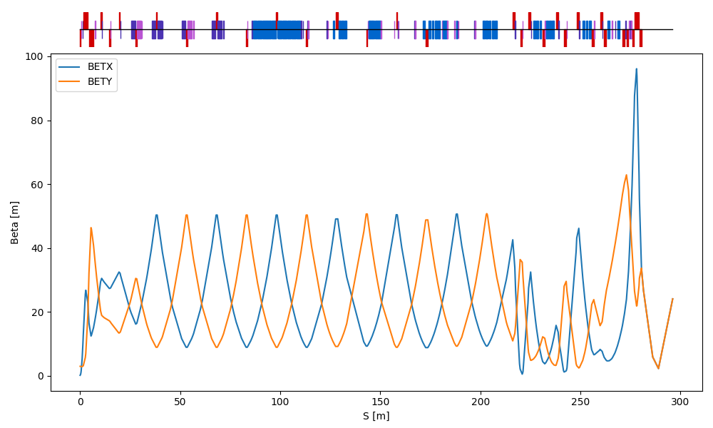
p.Beta()

This creates a plot of the Beta amplitude functions against curvilinear S position. A colour diagram representing the machine is also produced above the graph as shown below :

Other than beta, other optics plots can be made using Alpha(), Mu(), Disp() or Sigma(). These functions are provided as a quick utility and not the ultimate plotting script.

Machine lattice

The user can make their own plot and then append a machine diagram at the end if they wish :

f = matplotlib.pyplot.figure()
# user plotting commands here
pymad8.Plot.AddMachineLatticeToFigure(f, "mytwissfile")

gcf() is a matplotlib.pyplot function to get a reference to the current matplotlib figure and can be used as the first argument :

pymad8.Plot.AddMachineLatticeToFigure(gcf(), "mytwissfile")

Note

It becomes difficult to adjust the axes and layout of the graph after adding the machine description. It is therefore strongly recommended to do this last.

Colour Coding

Each magnet is colour coded an positioned depending on its type and strength.

Type	Shape	Colour	Vertical Position
drift	N/A	Not shown	N/A
sbend	Rectangle	Blue	Central always
rbend	Rectangle	Blue	Central always
hkicker	Rectangle	Purple	Central always
vkicker	Rectangle	Pink	Central always
quadrupole	Rectangle	Red	Top half for K1L > 0; Bottom half for K1L < 0
sextupole	Hexagon	Yellow	Central always
octupole	Hexagon	Green	Central always
multiple	Hexagon	Light grey	Central always
rcollimator	Rectangle	Black	Central always
ecollimator	Rectangle	Black	Central always
any other	Rectangle / Line	Light Grey	Central always

Note

In all cases if the element is a magnet and the appropriate strength is zero, it is shown as a grey line.