Collimation
Topcis Covered
Compare optics
Simulate beam loss
Analysis with filters
Use bdsim, rebdsim, pybdsim
Based on
bdsim/examples/collimation
Contents
Preparation
BDSIM has been compiled and installed.
The (DY)LD_LIBRARY_PATH and ROOT_INCLUDE_PATH environmental variables are set as described in Setup.
ROOT can be imported in Python
pybdsim has been installed.
Model Description
This is an example to show how to turn on extra collimation output and how to analyse the data. This example shows information most relevant to a collimation system. A basic version of this example exists that shows general data exploration and analysis (see Collimation). This example focusses on more detailed collimation specific information.
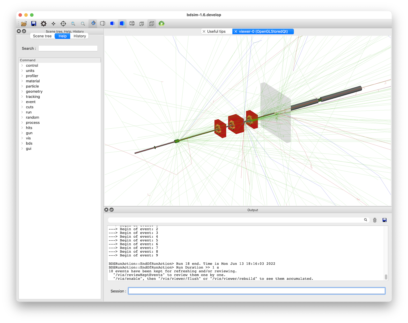
The model consists of two collimators, followed by a triplet set of quadrupoles, a shielding wall and a third collimator. The collimators are made of successively denser material (carbon, copper and tungsten). This looks like:
Model Preparation
The model is fictional and designed to show the relevant features of BDSIM. As the beam line was relatively short, the model was written by hand without any automatic conversion.
The files can be found in bdsim/examples/collimation:
collimation.gmad - model for beam losses and collimation
collimationOptics.gmad - model for Gaussian beam for optics
Optics
To understand how this machine transports particles, it is useful to
simulate a Gaussian beam that would nominally represent some ‘core’
beam that would be expected in the machine. Here we expect the losses
to be very low. A specific bdsim input file is included that chooses
a Gaussian distribution according to chosen Twiss parameters. Secondary
particles are stopped and the distribution is recorded after every
beam line element with the sample, all command. Running this
optics model takes around 10s to run 5000 particles on the developer’s
computer.:
bdsim --file=collimationOptics.gmad --outfile=o1 --batch --ngenerate=5000
Note
It is recommend to run at least 1000 particles for optical function evaluation and 10000 to 50000 if high accuracy is desired or a large energy spread is defined.
This produces an output file called “o1.root”. We can then calculate the optical functions and sizes of the beam after each element using the included rebdsimOptics tool.:
rebdsimOptics o1.root o1-optics.root
This creates another file called “o1-optics.root” that contains only the optical function information. The Python utility pybdsim can be used to visualise the data.:
ipython
>>> import pybdsim
>>> pybdsim.Plot.BDSIMOptics("o1-optics.root")
This produces a series of graphs showing, for example, the mean, sigma, divergence and dispersion of the beam. The sigma and dispersion are shown below.
Losses
Of course, more interesting than the optical functions is the possibility of beam losses. To illustrate this, we choose a beam distribution that is a circular ring of particles close to the edge of the collimator. Most will hit the first collimator but around 1/3 will make it through at the edges as the first collimator is square. We should generate some events to investigate the beam losses. The below command generates 2000 events (2000 primary particles), which takes approximately 30s on the developer’s computer.:
bdsim --file=collimation.gmad --outfile=data1 --batch --ngenerate=2000
This produces an output file called “data1.root”, which is approximately 20Mb. Firstly, we might like to quickly see if there were any losses at all and if there was any energy deposition. This can be done by browsing the output data file as described in Basic Data Inspection, however, we’d like to look at the average energy loss and impacts quickly. Histograms of the primary particle impact and loss points as well as energy deposition are included by default per event in the output. A tool for convenience (rebdsimHistoMerge) allows averaging of these quickly as opposed to running rebdsim with an analysis configuration text file. This is run as follows:
rebdsimHistoMerge data1.root data1-histos.root
This produces an output file called “data1-histos.root” that contains the merged histograms. This too can also be viewed with a TBrowser in ROOT as described in Basic Data Inspection, however, here we will make more standardised plots using pybdsim in Python.:
ipython
>>> import pybdsim
>>> pybdsim.Plot.LossAndEnergyDeposition("data1-histos.root", hitslegendloc='upper center')
>>> pybdsim.Plot.EnergyDeposition("data1-histos.root")
In the case of the first command, the legend overlaps with an expected data point, so we move it - this is optional (limitation of plotting library). These produce the following plots of primary hits, losses and energy deposition and secondly just energy deposition.
As expected we see a large fraction of particle impact the first collimator and we see some energy deposition throughout. Now, we can perform a more advanced analysis to learn about these impacts and losses in the collimation system.
Questions Answered
Question 1 Where are particles absorbed that impact the first collimator?
Question 2 Where do particles impact that don’t impact the first collimator?
Question 3 What secondaries make it through the shielding wall created from impacts on the first collimator?
Question 1
Where are particles absorbed that impact the first collimator?
We want to histogram the absorption point of the primary particle in each event but only for the events where the primary impact was in the first collimator. We always record the primary first hit point and the loss point, but here we make use of the collimator specific information. The first collimator is called “c1” and the collimator hits are stored under the “COLL_c1_0” branch of the Event tree.
Note
The name of the collimator is prefixed with “COLL_” to distinguish it from a sampler which would have the name “c1”. The suffix “_0” is because it’s the 0th placement of that collimator in the beam line.
In this collimator structure in the output there is a variable “primaryInteracted”. This
is a Boolean which is true if the primary particle interacted with the material of the
collimator on that event. We use this as a ‘selection’ in the histogram. We prepare
an analysis configuration text file for rebdsim (see Preparing an Analysis Configuration File).
We can start from an example in BDSIM and edit that one. An example can be found in
bdsim/examples/features/analysis/perEntryHistograms/analysisConfig.txt.
The variables in the histogram specification must be exactly as you see in the output file so it’s useful to use a TBrowser in ROOT to browse the file while preparing the analysis configuration file. The following is the desired histogram specification.:
# Object     treeName Histogram Name       #Bins Binning  Variable          Selection
Histogram1D  Event.   C1ImpactLossLocation {96}  {0:12}   PrimaryLastHit.S  COLL_c1_0.primaryInteracted
Note
Take note of the “.” in the variable names.
An example analysis configuration file is included in
bdsim/examples/collimation/analysisConfig.txt that contains the histograms
for this and subsequent questions.
This can be used with the following command:
rebdsim analysisConfig.txt data1.root data1-analysis.root
This produces a ROOT file called “data1-analysis.root” with the desired histograms. The
histograms are by default made ‘per event’ (i.e. the histogram is made separately for
each event, then these histograms are averaged), and the histogram “C1ImpactLossLocation”
will be in the Event/PerEntryHistograms/ directory in the file. This histogram
can be plotted with pybdsim.:
ipython
>>> from matplotlib.pyplot import *
>>> import pybdsim
>>> d = pybdsim.Data.Load("data1-analysis.root")
>>> d.histogramspy
{'Event/MergedHistograms/CollElossPE': <pybdsim.Data.TH1 at 0x119f90ad0>,
'Event/MergedHistograms/CollPInteractedPE': <pybdsim.Data.TH1 at 0x119f909d0>,
'Event/MergedHistograms/CollPhitsPE': <pybdsim.Data.TH1 at 0x119f90b10>,
'Event/MergedHistograms/CollPlossPE': <pybdsim.Data.TH1 at 0x119f90b90>,
'Event/MergedHistograms/ElossHisto': <pybdsim.Data.TH1 at 0x119f90c10>,
'Event/MergedHistograms/ElossPEHisto': <pybdsim.Data.TH1 at 0x119f90a10>,
'Event/MergedHistograms/PhitsHisto': <pybdsim.Data.TH1 at 0x119f90a50>,
'Event/MergedHistograms/PhitsPEHisto': <pybdsim.Data.TH1 at 0x119f82650>,
'Event/MergedHistograms/PlossHisto': <pybdsim.Data.TH1 at 0x119f90910>,
'Event/MergedHistograms/PlossPEHisto': <pybdsim.Data.TH1 at 0x119f90790>,
'Event/PerEntryHistograms/AfterShielding': <pybdsim.Data.TH2 at 0x119f90c90>,
'Event/PerEntryHistograms/C1ImpactLossLocation': <pybdsim.Data.TH1 at 0x119f90890>,
'Event/PerEntryHistograms/NoC1ImpactLossLocation': <pybdsim.Data.TH1 at 0x119f7d710>}
>>> pybdsim.Plot.Histogram1D(d.histogramspy['Event/PerEntryHistograms/C1ImpactLossLocation'])
>>> yscale('log', nonposy='clip')
>>> xlabel('S (m)')
>>> ylabel('Fraction of Primary Particles')
>>> pybdsim.Plot.AddMachineLatticeFromSurveyToFigure(gcf(), d.model)
Note
The y axis here is fraction of total events, so the integral of this histogram is not 1 as not all particle impact the first collimator. This is however, the accurate fraction of the events simulated, so this is what is required to correctly scale to a correct rate of expected events for this beam distribution.
The variable d.model is the beam line model included with each output file and automatically loaded with pybdsim.
the “nonposy=’clip’” argument to pyplot.yscale avoids gaps in the line of the histogram when plotting.
The command d.histogramspy is used to print out the numpy-converted histograms loaded from the file by pybdsim so that the name can be copied and pasted into the next command.
This shows that the particles that interact with the first collimator are lost (in order)
just after the c1 collimator in the beam pipe (*)
before the c1 collimator in the beam pipe (from back-scattering)
c2 collimator
c3 collimator
throughout the machine
Note
(*) We should remember the binning in this histogram does not break at the element boundaries so particles stopping both in the collimator and just afterwards in the collimator could be in the same bin. We can always look at the ‘per element’ histogram from the merged histograms.
When the machine diagram is added to the figure, a searching feature is activated. Right-clicking anywhere on the plot will print out in the Python terminal the nearest beam line element to that point. Here, we can right-click on any of the peaks to get the names of these beam line elements.
Question 2
Where do particles impact that don’t impact the first collimator?
Similarly, we want to histogram the impact location, so PrimaryFirstHit.S, but for only the events where the primary particle didn’t impact the first collimator. Again, we use a selection in the histogram specification.:
# Object     treeName Histogram Name       #Bins Binning  Variable           Selection
Histogram1D  Event.   NoC1ImpactLossLocation {96}  {0:12}  PrimaryFirstHit.S COLL_c1_0.primaryInteracted==0
This is included in the example analysis configuration
bdsim/examples/collimation/analysisConfig.txt that contains the histograms
for this and the other questions.
This can be used with the following command:
rebdsim analysisConfig.txt data1.root data1-analysis.root
Loading and plotting with pybdsim:
ipython
>>> from matplotlib.pyplot import *
>>> import pybdsim
>>> d = pybdsim.Data.Load("data1-analysis.root")
>>> d.histogramspy
{'Event/MergedHistograms/CollElossPE': <pybdsim.Data.TH1 at 0x119f90ad0>,
'Event/MergedHistograms/CollPInteractedPE': <pybdsim.Data.TH1 at 0x119f909d0>,
'Event/MergedHistograms/CollPhitsPE': <pybdsim.Data.TH1 at 0x119f90b10>,
'Event/MergedHistograms/CollPlossPE': <pybdsim.Data.TH1 at 0x119f90b90>,
'Event/MergedHistograms/ElossHisto': <pybdsim.Data.TH1 at 0x119f90c10>,
'Event/MergedHistograms/ElossPEHisto': <pybdsim.Data.TH1 at 0x119f90a10>,
'Event/MergedHistograms/PhitsHisto': <pybdsim.Data.TH1 at 0x119f90a50>,
'Event/MergedHistograms/PhitsPEHisto': <pybdsim.Data.TH1 at 0x119f82650>,
'Event/MergedHistograms/PlossHisto': <pybdsim.Data.TH1 at 0x119f90910>,
'Event/MergedHistograms/PlossPEHisto': <pybdsim.Data.TH1 at 0x119f90790>,
'Event/PerEntryHistograms/AfterShielding': <pybdsim.Data.TH2 at 0x119f90c90>,
'Event/PerEntryHistograms/C1ImpactLossLocation': <pybdsim.Data.TH1 at 0x119f90890>,
'Event/PerEntryHistograms/NoC1ImpactLossLocation': <pybdsim.Data.TH1 at 0x119f7d710>}
>>> pybdsim.Plot.Histogram1D(d.histogramspy['Event/PerEntryHistograms/NoC1ImpactLossLocation'])
>>> yscale('log', nonposy='clip')
>>> xlabel('S (m)')
>>> ylabel('Fraction of Primary Particles')
>>> pybdsim.Plot.AddMachineLatticeFromSurveyToFigure(gcf(), d.model)
Here we can see that particles that don’t impact the first collimator impact the second one and the third one. Some make it to the end of the beam line where they ‘hit’ the air of the world volume. Inspecting the raw data for Event.PrimaryFirstHit.S, we see some events with the value -1m. This is a value we put in the output when the impact was outside the curvilinear coordinate system, e.g. in the world volume away from the beam line. We can infer that the particles made it through the air of the world volume before reaching the boundary of the model.
Question 3
What secondaries make it through the shielding wall created from impacts on the first collimator?
We could plot many quantities of the secondary particles coming through the shielding wall, but, here we suggest the 2D flux. We therefore have a sampler attached to the “s1” beam line element (the shielding wall) that records in the distribution of all particles after it. We plot the 2D distribution of these particles and then filter them. The filter includes:
must be a secondary particle - parentID > 0
primary impact must be in c1 collimator - COLL_c1_0.primaryInteracted is true
This is the line added to the example analysis configuration file.:
# Object     treeName Histogram Name  #Bins   Binning             Variable  Selection
Histogram2D  Event.   AfterShielding  {50,50} {-2.5:2.5,-2.5:2.5} s1.y:s1.x COLL_c1_0.primaryInteracted&&s1.parentID>0
Note
Our analysis configuration file is a relatively thin interface to TTree::Draw in ROOT and so we see the inconsistency in ROOT for the order of the variables to be histogrammed. All of our specifications are x, then y, then z if further dimensions are required. However, with ROOT, the variable to be histogrammed is 1D: x, 2D y vs x, 3D x vs y vs z. The 2D variables are y:x here. The number of bins and ranges are in x, y, z order always.
This histogram can be plotted with pybdsim.:
ipython
>>> from matplotlib.pyplot import *
>>> import pybdsim
>>> d = pybdsim.Data.Load("data1-analysis.root")
>>> d.histogramspy
{'Event/MergedHistograms/CollElossPE': <pybdsim.Data.TH1 at 0x119f90ad0>,
'Event/MergedHistograms/CollPInteractedPE': <pybdsim.Data.TH1 at 0x119f909d0>,
'Event/MergedHistograms/CollPhitsPE': <pybdsim.Data.TH1 at 0x119f90b10>,
'Event/MergedHistograms/CollPlossPE': <pybdsim.Data.TH1 at 0x119f90b90>,
'Event/MergedHistograms/ElossHisto': <pybdsim.Data.TH1 at 0x119f90c10>,
'Event/MergedHistograms/ElossPEHisto': <pybdsim.Data.TH1 at 0x119f90a10>,
'Event/MergedHistograms/PhitsHisto': <pybdsim.Data.TH1 at 0x119f90a50>,
'Event/MergedHistograms/PhitsPEHisto': <pybdsim.Data.TH1 at 0x119f82650>,
'Event/MergedHistograms/PlossHisto': <pybdsim.Data.TH1 at 0x119f90910>,
'Event/MergedHistograms/PlossPEHisto': <pybdsim.Data.TH1 at 0x119f90790>,
'Event/PerEntryHistograms/AfterShielding': <pybdsim.Data.TH2 at 0x119f90c90>,
'Event/PerEntryHistograms/C1ImpactLossLocation': <pybdsim.Data.TH1 at 0x119f90890>,
'Event/PerEntryHistograms/NoC1ImpactLossLocation': <pybdsim.Data.TH1 at 0x119f7d710>}
>>> pybdsim.Plot.Histogram2D(d.histogramspy['Event/PerEntryHistograms/AfterShielding'], logNorm=True)
>>> xlabel('X (m)')
>>> ylabel('Y (m)')
>>> tight_layout()
The value plotted is the number of particles per square bin size on average per particle simulated including all the filters.
Note
The samplers by default are 5m wide, but may be shrunk to avoid geometrical overlaps in the case of a model with very large angle bends. Of course, this does not apply to this model.