Model Construction
The following sections describe the basics of how to prepare a BDSIM model.
Lattice Description
A model of the accelerator is given to BDSIM via input text files in the GMAD Syntax. The overall program structure should follow:
Component definition (see Beamline Elements)
Sequence definition using defined components (see Lattice Sequence)
Which sequence to use (see use - Defining which Line to Use)
Where to record output (see Output at a Surface - Samplers)
Options, including which physics lists, number to simulate etc. (see Options)
A beam definition (see Beam Parameters)
Specifying and option or definition again, will overwrite the previous value.
The only order specific part is the use command (see use - Defining which Line to Use) as this copied whatever sequence is used at that point, so any further updates to the component definitions will not be observed.
Apart from this, all other parts can be defined or redefined in any order in the input.
A beam line (using a sequence / line and the
usecommand are optional.
These are described in the following sections. Aside from these standard parameters, more detail may be added to the model through customisation - see Model Customisation.
Circular Machines
To simulate circular machines, BDSIM should be executed with the --circular executable option
(see Executable Options), or with the option, circular=1; in the input GMAD file. This
installs special beam line elements called the teleporter and terminator at the end of the lattice
that are described below.
Note
There must be a minimum \(0.2 \mu m\) gap between the last element and the beginning of the sequence to accommodate these elements. This has a minimal impact on tracking.
Both the terminator and teleporter are invisible and very thin elements that are not normally
shown in the visualiser. These can be visualised by executing BDSIM with the --vis_debug
executable option.
The turn number is automatically stored in the energy loss output in the data when the circular option is used.
Terminator
In a Geant4 / BDSIM model, all particles are tracked down to zero energy or until they leave the world volume. In the case of a circular accelerator, the particles may circulate indefinitely as they lose no energy traversing the magnetic fields. To control this behaviour and limit the number of turns taken in the circular machine, the terminator is inserted. This is a very thin disk that has dynamic limits attached to it. It is normally transparent to all particles and composed of vacuum. After the desired number of turns of the primary particle has elapsed, it switches to being an infinite absorber. It achieves this by setting limits (G4UserLimits) with a maximum allowed energy of 0eV.
The user should set the option nturns (default 1) (see Common Options).
option, nturns=56;
Teleporter
Not all optical models close perfectly in Cartesian coordinates, i.e. the ends don’t perfectly
align. Some small offsets may be tolerable, as most tracking codes use curvilinear coordinates.
To account for this, the teleporter is a small disk volume inserted to make up the space
and shift particles transversely as if the ends matched up perfectly. This is automatically
calculated and constructed when using the --circular executable option.
Although the teleporter may not be required in a well-formed model that closes, the minimum gap of \(0.2 \mu m\) is required for the terminator.
Beamline Starting Point
The main beamline, by default, starts at (X,Y,Z) = (0,0,0) and points in the
positive unit Z direction.
The initial position and direction of the baemline may be change with the options described in Offset for Main Beam Line.
Note
It should be noted that the beam or ‘bunch’ definition will move along with the beamline and the offset of the beam is with respect to this.
Magnet Strength Polarity
Note
BDSIM strictly follows the MAD-X definition of magnet strength parameter k - a positive k corresponds to horizontal focussing for a positively charged particle. This therefore indicates a positive k corresponds to horizontal defocussing for a negatively charged particle. However, MAD-X treats all particles as positively charged for tracking purposes.
Warning
BDSIM currently treats k absolutely, so to convert a MAD-X lattice for negatively particles, the MAD-X k values must be multiplied by -1. The pybdsim converter provides an option called flipmagnets for this purpose. This may be revised in future releases depending on changes to MAD-X.
Synchronous Time and Phase
Some components have time dependent fields, such as an rf cavity element. By default, these are given a synchronous global time in their construction so that local time is zero at the centre of the component for a synchronous particle. The time is calculated for a particle travelling at the speed of light from the start of the accelerator.
If the element is reused several times in a machine, it is constructed uniquely for each instance so that the fields are unique with their own synchronous time or phase.
Warning
This currently does not calculate the time based on the true velocity of the particle that may vary (with acceleration) throughout the accelerator. The speed of light in vacuum is used to calculate this time and the user should calculate an appropriate global tOffset for the component if the beam is sub-relativistic. This may be improved upon in future.
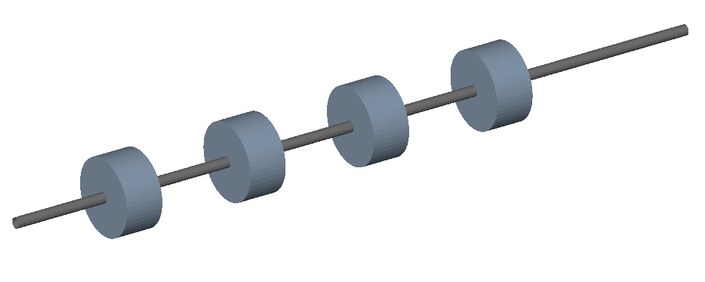
Beamline Elements
BDSIM provides a variety of different elements each with their own function, geometry and potential fields. Any element in BDSIM is described with the following pattern
name: type, parameter=value, parameter="string";
Note
Note the colon ‘:’ between name and type. The double (not single) inverted commas for a string parameter and that each functional line must end with a semi-colon. Spaces will be ignored.
The following elements may be defined
These are detailed in the following sections.
Simple example, extend and copy
Example:
d1: drift, l=5*m;
This defines a drift element with name d1 and a length of 5 metres. The definition can later be changed or extended with
d1: l=3*m, aper=0.1*m;
Note the omission of the type drift. This will change the length of d1 to 3 metres and set the aperture size to 10 centimetres.
Warning
This only works for beam line elements and not other objects in GMAD syntax (such as a placement).
An element can also be defined by copying an existing element
d2: d1, l=2*m;
Element d2 is a drift with the properties of d1 and a length of 2 metres. Note that if d1 is changed again, d2 will not change.
Component Strength Scaling
In the case of acceleration or energy degradation, the central energy of the beam may
change. However, BDSIM constructs all fields with respect to the rigidity calculated
from the particle species and the energy parameter in the beam definition (i.e. not the
central or mean energy of the beam E0, but the design energy given by energy).
To easily scale the strengths, every beam line element has the parameter scaling that enables
its strength to be directly scaled.
In the case of a dipole, this scales the field but not the angle (the field may be calculated from the angle if none is specified). For example
beam, particle="e-",
      energy=10*GeV;

sb1: sbend, l=2.5*m, angle=0.1;
d1: drift, l=1*m;
cav1: rf, l=1*m, gradient=50*MV/m, frequency=0;
sb2: sbend, l=2.5*m, angle=0.1, scaling=1.005;

l1: line=(sb1,d1,cav1,d1,sb2,d1);
In this example an rf cavity is used to accelerate the beam by 50 MeV (50 MV / m for 1 m). The particle passes through one bend, the cavity and then another. As the second bend is scaled (by a factor of (10 GeV + 50 MeV) / 10 GeV) = 1.005) a particle starting at (0,0) with perfect energy will appear at (0,0) after this lattice.
In the case of a quadrupole or other magnet, the scaling is internally applied to the k1 or appropriate parameter that is used along with the design rigidity to calculate a field gradient.
An example is included in examples/features/components/scaling.gmad.
Note
The user should take care to use this linear scaling parameter wisely- particularly in sub-relativistic regimes. The fields should typically be scaled with momentum and not total energy of the particle.
Magnet Yoke Field Scaling
As described in General Yoke Multipole, BDSIM uses by default an approximate magnetic field for the yoke or “outer” part of each magnet. This is a sum of infinite (in \(z\)) current sources placed in the \(x, y\) plane half way between each pole. This field is only approximate and field maps should be used if a very accurate model is desired.
These fields are normalised to match the vacuum field at the pole tip, so the transition is smooth.
However, to control this, an arbitrary scaling factor can be applied to all elements with a yoke field (i.e. all magnets). This can be applied individually, or as an option to all components. Individually specified parameters will take precedence.
In both cases the parameter and option is scalingFieldOuter and should be a numerical
factor (e.g. 1.0 is the default).
An example model is:
d1: drift, l=1*m;
q1: quadrupole, l=20*cm, k1=0.2, scalingFieldOuter=1.5;
q2: quadrupole, l=20*cm, k1=0.2;
l1: line=(d1,q1,d1,q2,d1);
use, l1;

beam, particle="proton", kineticEnergy=100*GeV;

option, scalingFieldOuter=2.0;
Here, the “q1” element will have an arbitrary scaling factor of the 1.5 over the normal field inside the pole tip radius. For “q2”, the default is picked up from the option with a value of 2.0.
This is recommended only for systematic error studies.
drift
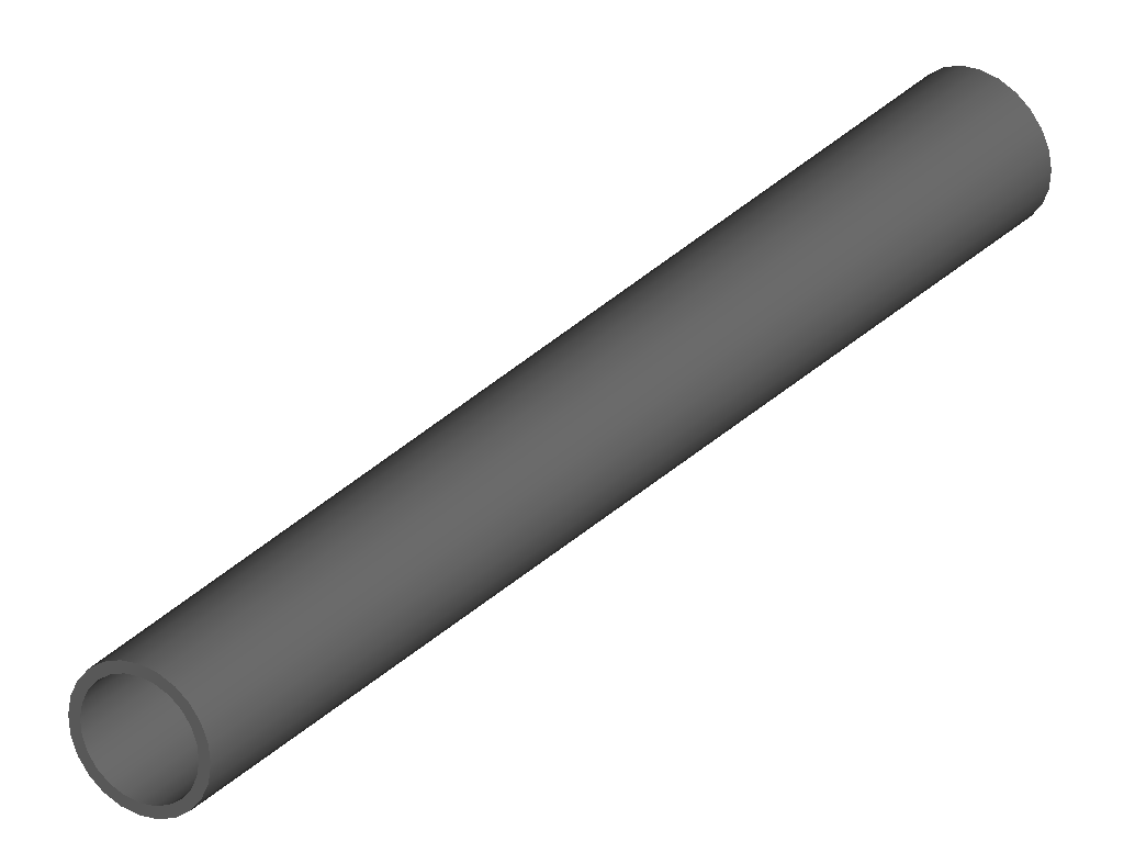
drift defines a straight beam pipe with no field.
Parameter |
Description |
Default |
Required |
l |
Length [m] |
0 |
Yes |
vacuumMaterial |
The vacuum material to use, can be user defined |
vacuum |
No |
Notes:
The Aperture Parameters may also be specified.
The default beam pipe material is “stainlessSteel”. This applies to all BDSIM elements that have a beam pipe.
Examples:
l203b: drift, l=1*m;
l204c: drift, l=3*cm, beampipeRadius=10*cm;
rbend
rbend defines a rectangular bend magnet. Either the total bending angle, angle, or the magnetic field, B, (in Tesla) for the nominal beam energy can be specified. If both are defined the magnet is under or over-powered. The faces of the magnet are normal to the chord of the input and output points. It can be specified using:
angle only - B calculated from the angle and the beam design rigidity.
B only - the angle is calculated from the beam design rigidity.
angle & B - physically constructed using the angle, and field strength as B (see also Component Strength Scaling).
Pole face rotations can be applied to both the input and output faces of the magnet, based upon the reference system shown in the figure below. A pure dipole field is provided in the beam pipe and a more general dipole (as described by General Yoke Multipole) is provided for the yoke. A quadrupolar component can be specified using the k1 parameter that is given by:
If k1 is specified, the integrator from the bdsimmatrix integrator set is used. This results in no physical pole face angle being constructed for tracking purposes. The tracking still includes the pole face effects.
Note
See Dipole Behaviour for important notes about dipole tracking.
Parameter |
Description |
Default |
Required |
|---|---|---|---|
l |
Chord Length [m] |
0 |
Yes |
angle |
Angle [rad] |
0 |
Yes, and or B |
B |
Magnetic field [T] |
0 |
Yes |
e1 |
Input pole face angle [rad] |
0 |
No |
e2 |
Output pole face angle [rad] |
0 |
No |
material |
Magnet outer material |
Iron |
No |
yokeOnInside |
Yoke on inside of bend |
0 |
No |
hStyle |
H style poled geometry |
0 |
No |
k1 |
Quadrupole coefficient for function magnet |
0 |
No |
fint |
Fringe field integral for the entrance face of the rbend |
0 |
No |
fintx |
Fringe field integral for the exit face of the rbend. -1 means default to the same as fint. 0 there will be no effect. |
-1 |
No |
fintK2 |
Second fringe field integral for the entrance face of the rbend |
0 |
No |
fintxK2 |
Second fringe field integral for the exit face of the rbend |
0 |
No |
hgap |
The half gap of the poles for fringe field purposes only |
0 |
No |
h1 |
Input poleface curvature \([m^{-1}]\) |
0 |
no |
h2 |
Output poleface curvature \([m^{-1}]\) |
0 |
no |
tilt |
Tilt of magnet [rad] |
0 |
no |
Notes:
The Aperture Parameters may also be specified.
The Magnet Geometry Parameters may also be specified.
Note
In the case that the lhcleft or lhcright magnet geometry types are used,
the yoke field will be a sum of two regular yoke fields at the LHC beam pipe
separation. The option yokeFieldsMatchLHCGeometry can be used to control
this. On by default.
Pole face notation for an rbend.
A few points about rbends:
For large angles (> 100 mrad), particles may hit the aperture, as the beam pipe is represented by a straight (chord) section and even nominal energy particles may hit the aperture, depending on the degree of tracking accuracy specified. In this case, consider splitting the rbend into multiple ones.
The pole face rotation angle is limited to \(\pm \pi /4\) radians.
If a non-zero pole face rotation angle is specified, the element preceding / succeeding the rotated magnet face must either be a drift or an rbend with opposite rotation (e.g. an rbend with \(e2 = 0.1\) can be followed by an rbend with \(e1 = -0.1\)). The preceding / succeeding element must be longer than the projected length from the rotation, given by \(2 \tan(\mathrm{eX})\).
Fringe field kicks are applied in a thin fringe field magnet (0.1 micron thick by default) at the beginning or at the end of the rbend. The length of the fringe field element can be set by the option thinElementLength (see Options) but is an advanced option.
In the case of finite fint or fintx and hgap, a fringe field is used even if e1 and e2 have no angle.
The fintK2 and fintxK2 parameters are for a second fringe field correction term that are included to enable optics comparisons with TRANSPORT. Whilst this term is not available in MAD-X, the default values of 0 mean this second fringe field correction will not be applied unless fintK2 or fintxK2 are explicitly specified as non-zero.
The effect of pole face rotations and fringe field kicks can be turned off for all dipoles by setting the option includeFringeFields=0 (see Options).
The poleface curvature does not construct the curved geometry. The effect is instead applied in the thin fringefield magnet.
rbends are limited in angle to less than \(\pi/2\).
A positive tilt angle corresponds to a clockwise rotation when looking along the beam direction as we use a right-handed coordinate system. A positive tilt angle of \(\pi/2\) for an rbend with a positive bending angle will produce a vertical bend where the beam is bent downwards.
The sign of the pole face rotations do not change when flipping the sign of the magnet bending angle. This is to match the behaviour of MAD-X; i.e. a positive pole face angle reduces the length of the outer side of the bend (the side furthest from the centre of curvature).
Examples:
MRB20: rbend, l=3*m, angle=0.003;
r1: rbend, l=5.43m, beampipeRadius=10*cm, B=2*Tesla;
RB04: rbend, l=1.8*m, angle=0.05, e1=0.1, e2=-0.1
sbend
sbend defines a sector bend magnet. Either the total bending angle, angle, or the magnetic field, B, (in Tesla) for the nominal beam energy can be specified. If both are defined the magnet is under or over-powered. The faces of the magnet are normal to the curvilinear coordinate system. It can be specified using:
angle only - B calculated from the angle and the beam design rigidity.
B only - the angle is calculated from the beam design rigidity.
angle & B - physically constructed using the angle, and field strength as B (see also Component Strength Scaling).
Pole face rotations can be applied to both the input and output faces of the magnet, based upon the reference system shown in the figure below. A pure dipole field is provided in the beam pipe and a more general dipole (as described by General Yoke Multipole) is provided for the yoke. A quadrupolar component can be specified using the k1 parameter that is given by:
If k1 is specified, the integrator from bdsimmatrix integrator set is used. This results in no physical pole face angle being constructed for tracking purposes. The tracking still includes the pole face effects.
The sbend geometry is constructed as many small straight sections with angled faces. This makes no effect on tracking, but allows a much higher variety of apertures and magnet geometry to be used given the Geant4 geometry. The number of segments is computed such that the maximum tangential error in the aperture is 1 mm.
With the default integrator set, the pole face rotations are not built into the geometry
such that the tracking will match MADX. If you use the geant4 integrator set,
the pole face geometry will be built fully.
Note
See Dipole Behaviour for important notes about dipole tracking.
Parameter |
Description |
Default |
Required |
|---|---|---|---|
l |
Arc length [m] |
0 |
Yes |
angle |
Angle [rad] |
0 |
Yes, and or B |
B |
Magnetic field [T] |
0 |
Yes |
e1 |
Input pole face angle [rad] |
0 |
No |
e2 |
Output pole face angle [rad] |
0 |
No |
material |
Magnet outer material |
Iron |
No |
yokeOnInside |
Yoke on inside of bend |
0 |
No |
hStyle |
H style poled geometry |
0 |
No |
k1 |
Quadrupole coefficient for function magnet |
0 |
No |
fint |
Fringe field integral for the entrance face of the sbend |
0 |
No |
fintx |
Fringe field integral for the exit face of the sbend. -1 means default to the same as fint. 0 there will be no effect. |
-1 |
No |
fintK2 |
Second fringe field integral for the entrance face of the sbend |
0 |
No |
fintxK2 |
Second fringe field integral for the exit face of the sbend |
0 |
No |
hgap |
The half gap of the poles for fringe field purposes only |
0 |
No |
h1 |
Input poleface curvature \([m^{-1}]\) |
0 |
no |
h2 |
Output poleface curvature \([m^{-1}]\) |
0 |
no |
tilt |
Tilt of magnet [rad] |
0 |
no |
Notes:
The Aperture Parameters may also be specified.
The Magnet Geometry Parameters may also be specified.
Note
In the case that the lhcleft or lhcright magnet geometry types are used,
the yoke field will be a sum of two regular yoke fields at the LHC beam pipe
separation. The option yokeFieldsMatchLHCGeometry can be used to control
this. On by default.
Pole face notation for an sbend.
A few points about sbends:
The pole face rotation angle is limited to \(\pm \pi /4\) radians.
If a non-zero pole face rotation angle is specified, the element preceding / succeeding the rotated magnet face must either be a drift or an sbend with the opposite rotation (e.g. an sbend with \(e2 = 0.1\) can be followed by an sbend with \(e1 = -0.1\)). The preceding / succeeding element must be longer than the projected length from the rotation, given by \(2 \tan(\mathrm{eX})\).
Fringe field kicks are applied in a thin fringe field magnet (0.1 micron thick by default) at the beginning or at the end of the sbend. The length of the fringe field magnet can be set by the option thinElementLength (see Options).
In the case of finite fint or fintx and hgap a fringe field is used even if e1 and e2 have no angle.
The fintK2 and fintxK2 parameters are for a second fringe field correction term that are included to enable optics comparisons with TRANSPORT. Whilst this term is not available in MAD-X, the default values of 0 mean this second fringe field correction will not be applied unless fintK2 or fintxK2 are explicitly specified as non-zero.
The effect of pole face rotations and fringe field kicks can be turned off for all dipoles by setting the option includeFringeFields=0 (see Options).
The poleface curvature does not construct the curved geometry. The effect is instead applied in the thin fringefield magnet.
Sbends are limited in angle to less than \(2\pi\). If the sbends are not split with the option
dontSplitSBends, an sbend will be limited in angle to a maximum of \(\pi/2\).A positive tilt angle corresponds to a clockwise rotation when looking along the beam direction as we use a right-handed coordinate system. A positive tilt angle of \(\pi/2\) for an sbend with a positive bending angle will produce a vertical bend where the beam is bent downwards.
The sign of the pole face rotations do not change when flipping the sign of the magnet bending angle. This is to match the behaviour of MAD-X; i.e. a positive pole face angle reduces the length of the outer side of the bend (the side furthest from the centre of curvature).
Examples:
s1: sbend, l=14.5*m, angle=0.005, magnetGeometryType="lhcright";
mb201x: sbend, l=304.2*cm, b=1.5*Tesla;
SB17A: sbend, l=0.61*m, angle=0.016, e1=-0.05, e2=0.09
quadrupole
quadrupole defines a quadrupole magnet. The strength parameter \(k_1\) is defined as
Parameter |
Description |
Default |
Required |
l |
Length [m] |
0 |
Yes |
k1 |
Quadrupole coefficient |
0 |
Yes |
material |
Magnet outer material |
Iron |
No |
Notes:
The Aperture Parameters may also be specified.
The Magnet Geometry Parameters may also be specified.
See Magnet Strength Polarity for polarity notes.
If lhcright or lhcleft magnet geometry types are used the yoke field is a sum of two as described in Multipole Yoke - Dual.
A pure quadrupolar field is provided in the beam pipe and a more general multipole (as described by General Yoke Multipole) is provided for the yoke.
Examples:
q1: quadrupole, l=0.3*m, k1=45.23;
qm15ff: quadrupole, l=20*cm, k1=95.2;
sextupole
sextupole defines a sextupole magnet. The strength parameter \(k_2\) is defined as
Parameter |
Description |
Default |
Required |
l |
Length [m] |
0 |
Yes |
k2 |
Sextupole coefficient |
0 |
Yes |
material |
Magnet outer material |
Iron |
No |
Notes:
The Aperture Parameters may also be specified.
The Magnet Geometry Parameters may also be specified.
See Magnet Strength Polarity for polarity notes.
If lhcright or lhcleft magnet geometry types are used the yoke field is a sum of two as described in ref:fields-multipole-outer-lhc.
A pure sextupolar field is provided in the beam pipe and a more general multipole (as described by General Yoke Multipole) is provided for the yoke.
Examples:
sx1: sextupole, l=0.5*m, k2=4.678;
sx2: sextupole, l=20*cm, k2=45.32;
octupole
octupole defines an octupole magnet. The strength parameter \(k_3\) is defined as
Parameter |
Description |
Default |
Required |
l |
Length [m] |
0 |
Yes |
k3 |
Octupole coefficient |
0 |
Yes |
material |
Magnet outer material |
Iron |
No |
Notes:
The Aperture Parameters may also be specified.
The Magnet Geometry Parameters may also be specified.
See Magnet Strength Polarity for polarity notes.
A pure octupolar field is provided in the beam pipe and a more general multipole (as described by General Yoke Multipole) is provided for the yoke.
Examples:
oct4b: octupole, l=0.3*m, k3=32.9;
decapole
decapole defines a decapole magnet. The strength parameter \(k_4\) is defined as
Parameter |
Description |
Default |
Required |
l |
Length [m] |
0 |
Yes |
k4 |
Decapole coefficient |
0 |
Yes |
material |
Magnet outer material |
Iron |
No |
A pure decapolar field is provided in the beam pipe and a more general multipole (as described by General Yoke Multipole) is provided for the yoke.
The Aperture Parameters may also be specified.
The Magnet Geometry Parameters may also be specified.
See Magnet Strength Polarity for polarity notes.
Examples:
MXDEC3: decapole, l=0.3*m, k4=32.9;
multipole
multipole defines a general multipole magnet. The strength parameter \(knl\) is a list defined as
starting with the quadrupole component. The skew strength parameter \(ksl\) is a list representing the skew coefficients.
Parameter |
Description |
Default |
Required |
l |
Length [m] |
0 |
Yes |
knl |
List of normal coefficients |
0 |
No |
ksl |
List of skew coefficients |
0 |
No |
material |
Magnet outer material |
Iron |
No |
Notes:
The values for knl and ksl are 1-counting, i.e. the first number is the order 1 component, which is the quadrupole coefficient.
The Aperture Parameters may also be specified.
The Magnet Geometry Parameters may also be specified.
See Magnet Strength Polarity for polarity notes.
No yoke field is provided.
Examples:
OCTUPOLE1 : multipole, l=0.5*m , knl={ 0,0,1 } , ksl={ 0,0,0 };
QUADRUPOLE1: multipole, l=20*cm, knl={2.3};
Note
If a multipole has a length equal to zero, it will be converted in a thinmultipole.
thinmultipole
thinmultipole is the same as multipole, but is set to have a default length of 0.1 micron. For thin multipoles, the length parameter is not required. The element will appear as a thin length of drift tube. A thin multipole can be placed next to a bending magnet with finite pole face rotation angles.
knl and ksl are the same as the thick multiple documented above. See multipole.
Examples:
THINOCTUPOLE1 : thinmultipole , knl={ 0,0,1 } , ksl={ 0,0,0 };
Note
The length of the thin multipole can be changed by setting thinElementLength (see Options).
vkicker
vkicker can either be a thin or thick vertical dipole magnet. If specified
with a finite length l, it will be constructed as a thick dipole. However, if no length (or
a length of exactly 0 is specified), a thin kicker will be built. In practice, the thin version is
constructed as a 0.1um slice with only the aperture geometry and no surrounding geometry and is not
visible with the default visualisation settings.
The strength is specified by the parameter vkick, which is the fractional momentum kick
in the vertical direction. A positive value corresponds to an increase in \(p_y\). In the
case of the thin kicker the position is not affected, whereas with the thick kicker, the position
will change.
The strength may also be specified by the magnetic field B. A positive field value corresponds
to an increase in \(p_y\) for a positively charged particle.
Warning
vkick will supersede the strength even if B is specified. Therefore, the
user should specify only vkick or B.
In the case of a thick vertical kicker, the resulting bending angle is calculated using:
where \(p_y\) is the fractional change in vertical momentum. The dipole field strength is then calculated with respect to the chord length:
For thin kickers, the magnetic field B is ignored and the element is treated as a drift.
The Aperture Parameters may also be specified.
For a vkicker with a finite length, the Magnet Geometry Parameters may also be specified.
Note
Pole face rotations and fringe fields can be applied to vkickers by supplying the same parameters that would be applied to an rbend or sbend . If the vkicker is zero length, the B field value must be supplied in order to calculate the bending radius which required to apply the effects correctly.
Fringe field kicks are applied in a thin fringe field magnet (0.1 micron thick by default) at the beginning or at the end of the vkicker. The length of the fringe field element can be set by the option thinElementLength (see Options).
For zero length vkickers, the pole face and fringe field kicks are applied in the same thin element as the vkick.
In the case of finite fint or fintx and hgap, a fringe field is used even if e1 and e2 have no angle.
The effect of pole face rotations and fringe field kicks can be turned off for all magnets by setting the option includeFringeFields=0 (see Options).
No pole face geometry is constructed.
A pure dipole field is provided in the beam pipe and a more general multipole (as described by General Yoke Multipole) is provided for the yoke.
Examples:
KX15v: vkicker, vkick=1.3e-5;
KX17v: vkicker, vkick=-2.4e-2, l=0.5*m;
KX18v: vkicker, B=0.04*T;
hkicker
hkicker can either be a thin horizontal kicker or a thick horizontal dipole magnet. If
specified with a finite length l, it will be constructed as a dipole. However, if no length (or
a length of exactly 0) is specified, a thin kicker will be built. This is typically a 0.1um slice
with only the shape of the aperture and no surrounding geometry. It is also typically not
visible with the default visualisation settings.
The strength is specified by the parameter hkick, which is the fractional momentum kick
in the vertical direction. A positive value corresponds to an increase in \(p_x\). In the
case of the thin kicker the position is not affected, whereas with the thick kicker, the position
will change.
The strength may also be specified by the magnetic field B. A positive field value corresponds
to an decrease in \(p_x\) (note right-handed coordinate frame) for a positively charged particle.
Warning
hkick will supersede the strength even if B is specified. Therefore, the
user should specify only hkick or B.
Note
A positive value of hkick causes an increase in horizontal momentum, so the particle will bend to the left looking along the beam line, i.e. in positive x. This is the opposite of a bend where a positive angle causes a deflection in negative x.
For thin kickers, the magnetic field B is ignored and the element is treated as a drift.
The Aperture Parameters may also be specified.
For a hkicker with a finite length, the Magnet Geometry Parameters may also be specified.
Note
Pole face rotations and fringe fields can be applied to hkickers by supplying the same parameters that would be applied to an rbend or sbend . If the hkicker is zero length, the B field value must be supplied in order to calculate the bending radius which required to apply the effects correctly.
Fringe field kicks are applied in a thin fringe field magnet (0.1 micron thick by default) at the beginning or at the end of the hkicker. The length of the fringe field element can be set by the option thinElementLength (see Options).
For zero length hkickers, the pole face and fringe field kicks are applied in the same thin element as the hkick.
In the case of finite fint or fintx and hgap, a fringe field is used even if e1 and e2 have no angle.
The effect of pole face rotations and fringe field kicks can be turned off for all magnets by setting the option includeFringeFields=0 (see Options).
No pole face geometry is constructed.
A pure dipole field is provided in the beam pipe and a more general multipole (as described by General Yoke Multipole) is provided for the yoke.
Examples:
KX17h: hkicker, hkick=0.01;
KX19h: hkicker, hkick=-1.3e-5, l=0.2*m;
KX21h: hkicker, B=0.03*T;
kicker
kicker defines a combined horizontal and vertical kicker. Either both or one of the parameters hkick and vkick may be specified. Like the hkicker and vkicker, this may also be thin or thick. In the case of the thick kicker, the field is the linear sum of two independently calculated fields.
Note
Pole face rotation and fringe fields kicks are unavailable for plain kickers
Example:
kick1: kicker, l=0.45*m, hkick=1.23e-4, vkick=0.3e-4;
tkicker
BDSIM, like MAD-X, provides a tkicker element. This is an alias in BDSIM for a kicker, however MAD-X differentiates the two on the basis of fitting parameters. BDSIM does not make this distinction. See kicker for more details.
In the case of a tkicker, the field B cannot be used and only hkick and vkick
can be used.
Note
Pole face rotation and fringe fields kicks are unavailable for tkickers
rf
rf or rfcavity defines an RF cavity with a time varying electric or electromagnetic field. There are several geometry and field options as well as ways to specify the strength. The default field is a uniform (in space) electric-only field that is time varying according to a cosine (see Sinusoidal Electric Field). Optionally, the electromagnetic field for a pill-box cavity may be used (see Pill-Box Cavity). The G4ClassicalRK4 numerical integrator is used to calculate the motion of particles in both cases. Fringes for the edge effects are provided by default and are controllable with the option includeFringeFieldsCavities.
Parameter |
Description |
Default |
Required |
|---|---|---|---|
l |
Length [m] |
0 |
Yes |
E |
Voltage [V] that will be across the length l |
0 |
Yes (or gradient) |
gradient |
Electric field [V/m] |
0 |
Yes (or E) |
frequency |
Frequency of oscillation (Hz) |
0 |
Yes |
phase |
Phase offset (rad) |
0 |
No |
tOffset |
Offset in time (s) |
0 |
No |
material |
Outer material |
“” |
Yes |
cavityModel |
Name of cavity model object |
“” |
No |
Either gradient or E should be specified. E (the voltage is given in Volts,
and internally is divided by the length of the element (l) to give the electric
field in Volts/m. If gradient is specified, this is already Volts/m and the length
is not involved. The slight misnomer of E instead of say voltage is historical.
Units Since the value of m as a unit in GMAD is 1.0, it doesn’t practically make a
difference whether you write gradient=10*MV/m or gradient=10*MV. However,
it is best to be explicit in units or none at all and assume the default ones.
Note
The design energy of the machine is not affected, so the strength and fields of components after an RF cavity in a lattice are calculated with respect to the design energy, the particle and therefore, design rigidity. The user should scale the strength values appropriately if they wish to match the increased momentum of the particle.
Warning
The elliptical cavity geometry may not render or appear in the Geant4 QT visualiser. The geometry exists and is valid, but this is due to deficiencies of the Geant4 visualisation system. The geometry exists and is fully functional.
The field is such that a positive E-field results in acceleration of the primary particle (depending on the primary particle charge).
The phase is calculated automatically such that zero phase results in the peak E-field at the centre of the component for its position in the lattice.
Either tOffset or phase may be used to specify the phase of the oscillator.
The material must be specified in the rf gmad element or in the attached cavity model by name. The cavity model will override the element material.
The entrance / exit cavity fringes are not constructed if the previous / next element is also an rf cavity.
The cavity fringe element is by default the same radius as the beam pipe radius. If a cavity model is supplied, the cavity fringes are built with the same radius as the model iris radius.
If phase is specified, this is added to the calculated phase offset from either the lattice position or tOffset.
The step length in the cavity is limited for all particles to be 2.5% of the minimum of the element length and the wavelength (given the frequency). In the case of 0 frequency, only the length is considered. This is to ensure accurate numerical integration of the motion through the varying field.
If tOffset is specified, a phase offset is calculated from this time for the speed of light in a vacuum. Otherwise, the curvilinear S-coordinate of the centre of the rf element is used to find the phase offset.
In the case where frequency is not set, the phase offset is ignored and only the phase is used. See the developer documentation Sinusoidal Electric Field for a description of the field.
Note
As the phase offset is calculated from the speed of light in a vacuum, this is only correct for already relativistic beams. Development is underway to improve this calculation for sub-relativistic beams.
Simple examples:
rf1: rf, l=10*cm, E=10*MV, frequency=90*MHz, phase=0.02;
rf2: rf, l=10*cm, gradient=14*MV/m, frequency=450*MHz;
rf3: rf, l=10*cm, E=10*MV, frequency=90*MHz, tOffset=3.2*ns;
Rather than just a simple E-field, an electromagnetic field that is the solution to a cylindrical pill-box cavity may be used. A cavity object (described in more detail below) is used to specify the field type. All other cavity parameters may be safely ignored and only the field type will be used. The field is described in Pill-Box Cavity.
Pill-box field example:
rffield: field, type="rfcavity";
rf4: rf, l=10*cm, E=2*kV, frequency=1.2*GHz, fieldVacuum="rffield";
Elliptical SRF cavity geometry is also provided and may be specified by use of another ‘cavity’ object in the parser. This cavity object can then be attached to an rf object by name. Details can be found in Cavity Geometry Parameters.
rfx & rfy
rfx or rfy define an RF cavity with a time varying electric (only) field that is transverse to the S direction the accelerator is built along. Particularly, for rfx it is in the local x direction and for rfy it is in the local y direction. The cavity will look like a cylindrical pillbox cavity much the same way as rf.
A positive gradient or field value causes a positive deflection in that direction.
Only gradient can be specified because if we specify voltage only, we need the length to calculate a gradient for the electric field and the exact width of the cavity can be ambiguous given a combination of parameters.
Parameter |
Description |
Default |
Required |
|---|---|---|---|
l |
Length [m] |
0 |
Yes |
gradient |
Electric field [V/m] |
0 |
Yes |
frequency |
Frequency of oscillation (Hz) |
0 |
Yes |
phase |
Phase offset (rad) |
0 |
No |
tOffset |
Offset in time (s) |
0 |
No |
material |
Outer material |
“” |
Yes |
See rf for details about phase and tOffset. The field is the same as Sinusoidal Electric Field, but pointing transversely.
Examples:
rf1: rfx, l=20*cm, gradient=12*MV / m, frequency=450*MHz;
target
A target defines a block of 1 material. By default, a square shape is used but a circular one can also be used. A target can be achieved similarly with an rcol with no xsize or ysize specified.
Parameter |
Description |
Default |
Required |
|---|---|---|---|
l |
Length [m] |
0 |
Yes |
material |
Outer material |
None |
Yes |
horizontalWidth |
Outer full width [m] |
0.5 m |
No |
colour |
Name of colour desired for block See Colours |
“” |
No |
minimumKineticEnergy |
Minimum kinetic energy below which to artificially kill particles in this target only |
0 |
No |
apertureType |
Temporarily used to describe the outer shape - only “circular” or “rectangular” are accepted |
“rectangular” |
No |
In future, apertureType will not be used to control the outer shape and any shape will be possible.
rcol
An rcol defines a rectangular collimator. The aperture is rectangular and the external volume is square.
If no xsize or ysize are provided, they are assumed to be 0 and a solid block is made.
Parameter |
Description |
Default |
Required |
|---|---|---|---|
l |
Length [m] |
0 |
Yes |
xsize |
Horizontal half aperture [m] |
0 |
Yes |
ysize |
Vertical half aperture [m] |
0 |
Yes |
material |
Outer material |
None |
Yes |
horizontalWidth |
Outer full width [m] |
0.5 m |
No |
xsizeOut |
Horizontal exit half aperture [m] |
xsize value |
No |
ysizeOut |
Vertical exit half aperture [m] |
ysize value |
No |
colour |
Name of colour desired for block See Colours |
“” |
No |
minimumKineticEnergy |
Minimum kinetic energy below which to artificially kill particles in this collimator only |
0 |
No |
Notes:
horizontalWidth should be big enough to encompass the xsize and ysize.
The parameter minimumKineticEnergy (in GeV by default) may be specified to artificially kill particles below this kinetic energy in the collimator. This is useful to match other simulations where collimators can be assumed to be infinite absorbers. If this behaviour is required, the user should specify an energy greater than the total beam energy.
The collimator can be tapered by specifying an exit aperture size with xsizeOut and ysizeOut, with the xsize and ysize parameters defining the entrance aperture.
All collimators can be made infinite absorbers with the general option
collimatorsAreInfiniteAbsorbers(see Tracking Options).
Examples:
! Standard
TCP15: rcol, l=1.22*m, material="graphite", xsize=104*um, ysize=5*cm;

! Tapered
TCP16: rcol, l=1.22*m, material="graphite", xsize=104*um, ysize=5*cm, xsizeOut=208*um, ysizeOut=10*cm;
! with kinetic energy limit
TCP6CD: rcol, l=0.6*m, material="C", xsize=200*um, ysize=5*cm, minimumKineticEnergy=10*MeV;
Note
The outer shape of an rcol can be made circular by defining apertureType="circular" for
that specific element. This is a temporary facility and may cause overlaps if the
horizontalWidth parameter is smaller than the radius from the xsize and ysize
parameters. In future this will be improved and generalised for any inner and outer shape. No
other outer shapes are supported just now.
Example:
r1: rcol, l=1*m, material="Cu", xsize=10*mm, ysize=3*mm, apertureType="circular", horizontalWidth=10*cm;
ecol
ecol defines an elliptical collimator. This is exactly the same as rcol except that the aperture is elliptical and the xsize and ysize define the horizontal and vertical half-axes respectively.
A circular aperture collimator can be achieved by setting xsize and ysize to the same value.
When tapered, the ratio between the horizontal and vertical half-axes of the entrance aperture (xsize and ysize) must be the same ratio for the exit aperture (xsizeOut and ysizeOut).
All the same conditions for rcol apply for ecol.
jcol
jcol defines a jaw collimator with two square blocks on either side in the horizontal plane. If a vertical jcol is required, the tilt parameter should be used to rotate it by \(\pi/2\). The horizontal position of each jaw can be set separately with the xsizeLeft and xsizeRight apertures which are the distances from the centre of element to the left and right jaws respectively. The collimator jaws can be individually tilted in a plane perpendicular to the jaw opening plane with the jawTiltLeft and jawTiltRight arguments. In this case, the set aperture is in the middle of the collimator. This feature can be useful for example in aligning the jaws to the beam envelope.
Parameter |
Description |
Default |
Required |
|---|---|---|---|
l |
Length [m] |
0 |
Yes |
xsize |
Horizontal half aperture [m] |
0 |
Yes |
ysize |
Half height of jaws [m] |
0 |
Yes |
material |
Outer material |
None |
Yes |
xsizeLeft |
Left jaw aperture [m] |
0 |
No |
xsizeRight |
Right jaw aperture [m] |
0 |
No |
jawTiltLeft |
Left jaw tilt angle [rad] |
0 |
No |
jawTiltRight |
Right jaw tilt angle [rad] |
0 |
No |
horizontalWidth |
Outer full width [m] |
0.5 m |
No |
colour |
Name of colour desired for block. See Colours. |
“” |
No |
minimumKineticEnergy |
Minimum kinetic energy below which to artificially kill particles in this collimator only |
0 |
No |
Notes:
The horizontalWidth must be greater than 2x xsize.
To prevent the jaws overlapping with one another, a jaw cannot be constructed that crosses the X axis of the element (i.e supplying a negative xsizeLeft or xsizeRight will not work). Should you require this, please offset the element using the element parameters offsetX and offsetY instead.
To construct a collimator jaws with one jaw closed (i.e. an offset of 0), the horizontal half aperture must be set to 0, with the other jaws half aperture set as appropriate.
If xsize, xsizeLeft and xsizeRight are not specified, the collimator will be constructed as a box with no aperture.
For only one jaw, specifying a jaw aperture which is larger than half the horizontalWidth value will result in that jaw not being constructed. If both jaw apertures are greater than half the horizontalWidth, no jaws will be built and BDSIM will exit.
To preserve the longitudinal dimensions, jaw tilt specified with jawTiltLeft or jawTiltRight and xsizeRight uses parallelepipeds instead of boxes for the collimator jaws. Relative to using angled boxes, this can introduce and error in the material traversed by incident particles, which scales as $btan(alpha)$, where b is the impact parameter (depth of impact) and $alpha$ is the jaw tilt angle.
The parameter minimumKineticEnergy (GeV by default) may be specified to artificially kill particles below this kinetic energy in the collimator. This is useful to match other simulations where collimators can be assumed to be infinite absorbers. If this behaviour is required, the user should specify an energy greater than the total beam energy.
All collimators can be made infinite absorbers with the general option
collimatorsAreInfiniteAbsorbers(see Tracking Options).
Examples:
! standard
TCP15: jcol, l=1.22*m, material="graphite", xsize=0.1*cm, ysize=5*cm;

! two separately specified jaws
j1: jcol, l=1*m, horizontalWidth=1*m, material="Cu", xsizeLeft=1*cm, xsizeRight=1.5*cm;

! only left jaw
j2: jcol, l=0.9*m, horizontalWidth=1*m, material="Cu", xsizeLeft=1*cm, xsizeRight=2*m;
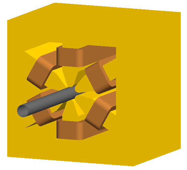
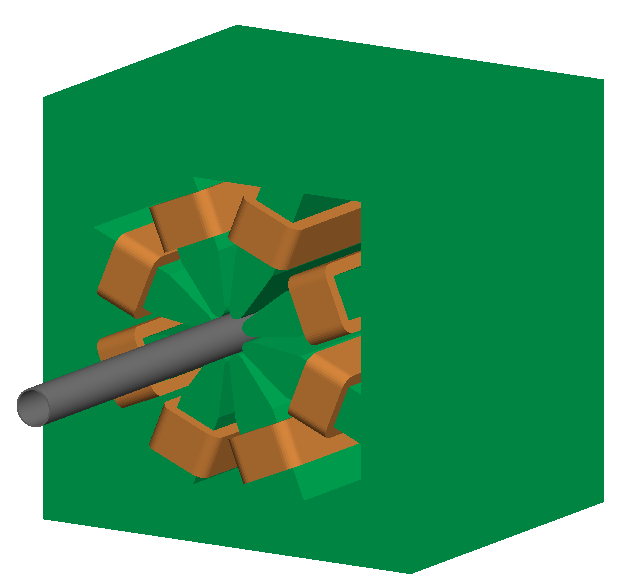
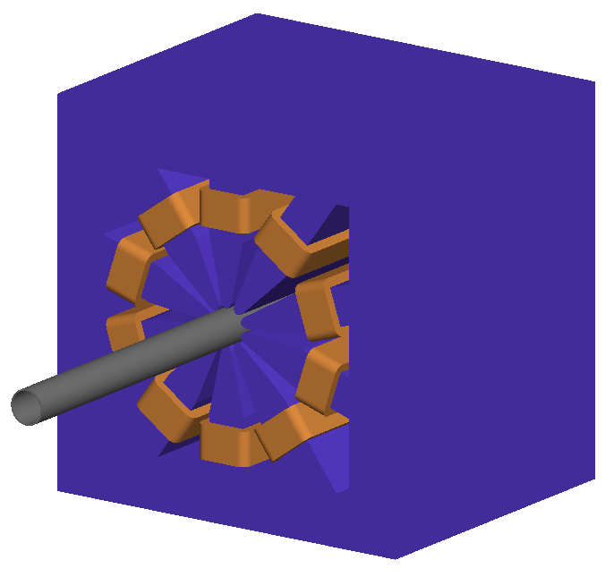
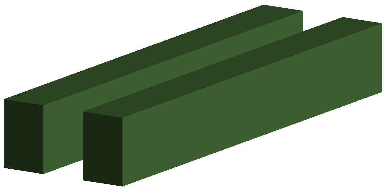
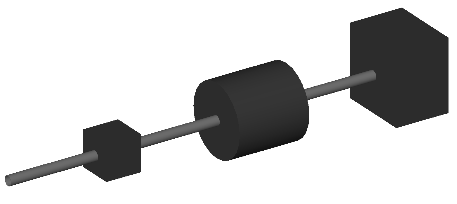
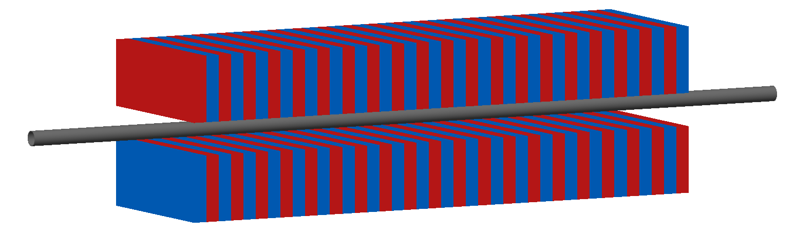
degrader
degrader defines interleaved pyramidal pieces of material. Depending on the physics list used, this is capable of reducing the beam energy. This happens only through interaction and the use of a physics list. Note, the default physics list in BDSIM is no physics and only magnetic tracking, in which case this component will have no effect.
If 1 wedge is specified, the degrader will be composed of 1 half wedge on each side.
If 2 wedges are specified, the degrader will be a half, a whole then a half wedge.
The above diagram shows a degrader with 3 wedges specified.
Warning
The nominal beam energy of each magnet after the degrader is unchanged and
is still the design energy of the machine. It is not possible to accurately
calculate the degradation in kinetic energy for all materials and particles
analytically. The user should use the scaling parameter for any
magnet placed after the degrader to linearly scale the field strength. Or in
the case where there are no magnets before the degrader, set the design energy
of using the beam command as the energy afterwards and the E0 to the
higher input energy.
Parameter |
Description |
Default |
Required |
l |
Length [m] |
0 |
Yes |
numberWedges |
Number of degrader wedges |
1 |
Yes |
wedgeLength |
Degrader wedge length [m] |
0 |
Yes |
degraderHeight |
Degrader height [m] |
0 |
Yes |
materialThickness |
Amount of material seen by the beam [m] |
0 |
Yes/No* |
degraderOffset |
Horizontal offset of both wedge sets |
0 |
Yes/No* |
material |
Degrader material |
Carbon |
Yes |
horizontalWidth |
Outer full width [m] |
global |
No |
colour |
Colour of block. See Colours |
“” |
No |
Note
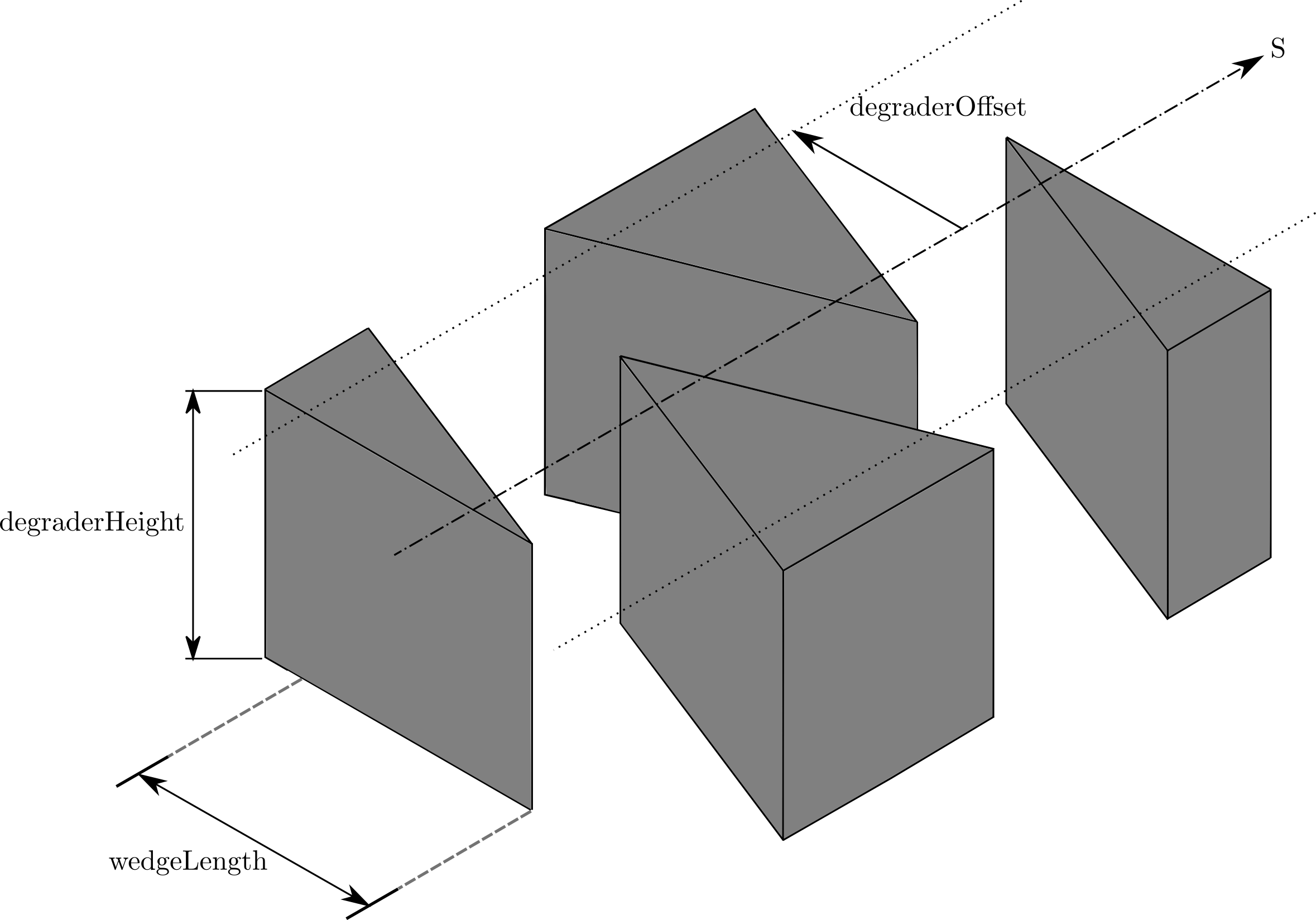
Either materialThickness or degraderOffset can be specified to adjust the horizontal lateral wedge position, and consequently the total material thickness the beam can propagate through. An offset of zero will corresponds to a full closed degrader, and is equivalent to a materialThickness being the degrader length. If both are specified, degraderOffset will be ignored.
Note
When numberWedges is specified to be n, the degrader will consist of n-1 full wedges and two half wedges. When viewed from above, a full wedge appears as an isosceles triangle, and a half wedge appears as a right-angled triangle.
Note
A base is included with each wedge. Without it, if the materialThickness were to be set to the same as the degrader length, only half the beam would be degraded when passing through a wedge. The base provides material such that the whole width of the beam pipe would see material when the degrader is fully closed. As such, the degrader offset must be greater than or equal to zero. Negative offsets causes BDSIM to exit.
Note
If the user wants a fully open degrader, the degrader offset should be set to a value larger than the wedgeLength.
Examples:
DEG1: degrader, l=0.25*m, material="carbon", numberWedges=5, wedgeLength=100*mm, degraderHeight=100*mm, materialThickness=200*mm;
DEG2: degrader, l=0.25*m, material="carbon", numberWedges=5, wedgeLength=100*mm, degraderHeight=100*mm, degraderOffset=50*mm;
muspoiler
muspoiler defines a muon spoiler, which is a rotationally magnetised iron cylinder with a beam pipe in the middle. There is no magnetic field in the beam pipe.
Parameter |
Description |
Default |
Required |
l |
Length [m] |
0 |
Yes |
B |
Magnetic field [T] |
0 |
No |
material |
Outer material |
Iron |
No |
horizontalWidth |
Outer full width [m] |
global |
No |
Notes:
The Aperture Parameters may also be specified.
No field is constructed if B is the default 0.
shield
shield defines a square block of material with a square aperture. The user may choose the outer width and inner horizontal and vertical apertures of the block. A beam pipe is also placed inside the aperture. If the beam pipe dimensions (including thickness) are greater than the aperture, the beam pipe will not be created.
Parameter |
Description |
Default |
Required |
l |
Length [m] |
0 |
Yes |
material |
Outer material |
Iron |
No |
horizontalWidth |
Outer full width [m] |
global |
No |
xsize |
Horizontal inner half aperture [m] |
0 |
Yes |
ysize |
Vertical inner half aperture [m] |
0 |
No |
colour |
Colour of block. See Colours |
“” |
No |
Notes:
The Aperture Parameters may also be specified.
dump
dump defines a square or circular block of material that is an infinite absorber. All particles impacting the dump will be absorbed irrespective of the particle and physics processes.
This is intended as a useful way to absorb a beam with no computational time. Normally, the world volume is filled with air. If the beam reaches the end of the beam line it will hit the air and likely create a shower of particles that will take some time to simulate. In this case, when this isn’t required, it is recommended to use a dump object to absorb the beam.
Parameter |
Description |
Default |
Required |
l |
Length [m] |
1 mm |
No |
horizontalWidth |
Outer full width [m] |
global |
No |
apertureType |
Which shape |
rectangular |
No |
How this works: the material of the dump is actually vacuum, but G4UserLimits are used to kill particles. This requires the cuts and limits physics process that is included automatically. In the case of using a Geant4 reference physics list (see Geant4 Reference Physics Lists), the necessary process is added automatically to enforce this.
The dump may accept apertureType with the value of either circular or rectangular for the shape of the dump. By default it is rectangular.
Note
Although the syntax is “rectangular”, the shape for the dump will be square. This will be improved in future when any shape can be used.
Examples:
d1: dump, horizontalWidth=20*cm;
d2: dump, horizontalWidth=30*cm, apertureType="circular";
d3: dump, l=0.3*m, horizontalWidth=40*cm, apertureType="rectangular";
Here, d1 is a rectangular block 20 cm wide (full width) and 1 mm long in z. d2 is a circular disk with diameter 30 cm and length of 1 mm in z. d3 is 30 cm long in z and 40 cm width (full width) in x and y with a square shape.
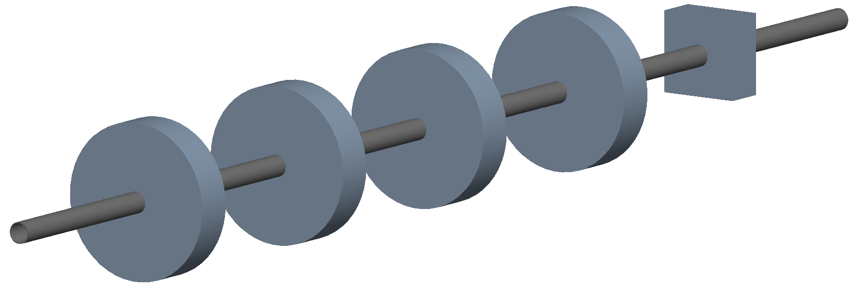
solenoid
solenoid defines a solenoid magnet. This utilises a thick lens transfer map with a hard edge field profile. Fringes for the edge effects are provided by default and are controllable with the option includeFringeFields. A field is supplied that is used in the case a particle cannot be tracked using the integrator. In this case, it is a perfect dipole field along the local \(z\) axis inside the beam pipe with no spatial variation. Outside the beam pipe, in the ‘yoke’, a solenoidal field according to a cylindrical current source is constructed.
Parameter |
Description |
Default |
Required |
l |
Length [m] |
0 |
Yes |
ks |
Solenoid strength |
0 |
No |
B |
Magnetic field |
0 |
No |
material |
Outer material |
Iron |
No |
horizontalWidth |
Outer full width [m] |
global |
No |
A positive field corresponds to a field in along the direction of positive S.
The entrance / exit solenoid fringes are not constructed if the previous / next element is also a solenoid.
See Magnet Strength Polarity for polarity notes.
A thin sheet cylinder is place also inside the yoke but of the same material. The colour is copper colour to indicate this is the shape used to calculate the solenoidal field for the yoke. This is of the same material so it has no effect on physics results. The ‘current’ cylinder is chosen to be \(0.8 \times l\) and the radius is \(\frac{1}{3}\) of the distance between the beam pipe radius and the outer radius.
Examples:
atlassol: solenoid, l=20*m, ks=0.004;
Another visualisation:
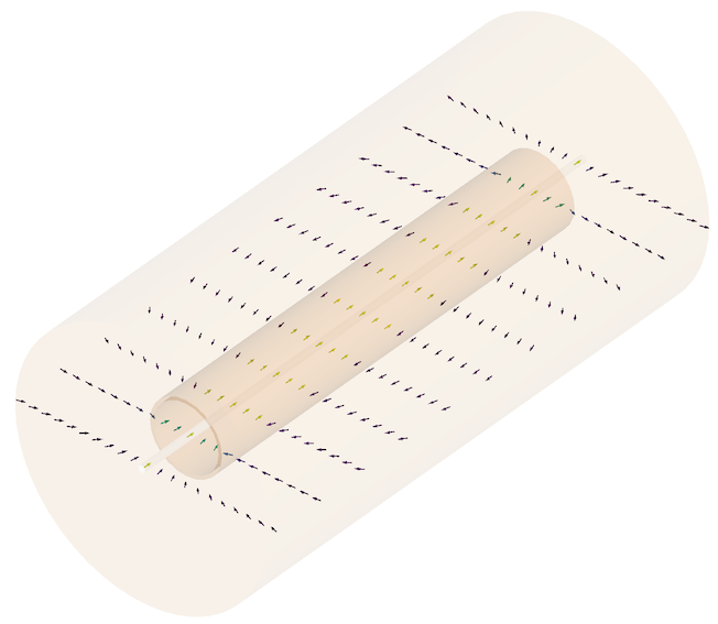
A partially transparent visualiation of a solenoid showing the interior current cylinder sheet - made of the same material as the yoke. The field is shown in the \(x-z\) plane.
wirescanner
wirescanner defines a cylindrical object within a beam pipe to represent a wire scanner typically use in an accelerator.
parameter |
description |
default |
required |
l |
length of drift section around wire |
0 |
yes |
wireDiameter |
diameter of wire [m] |
0 |
yes |
wireLength |
length of wirescanner [m] |
0 |
yes |
material |
material of wire |
none |
yes |
wireAngle |
angle of the wire w.r.t. vertical |
0 |
no |
wireOffsetX |
x offset of the wire from the center [m] |
0 |
no |
wireOffsetY |
y offset of the wire from the center [m] |
0 |
no |
wireOffsetZ |
z offset of the wire from the center [m] |
0 |
no |
Notes:
The angle is the rotation from vertical in the clock-wise direction looping in the positive S direction (the usually direction of the beam).
Warning
After BDSIM V1.3.2 wireAngle is used for the angle instead of
angle as angle is used specifically for angles of bends
and this could result in the curvilinear world being made very small.
The offsets are with respect to the centre of the beam pipe section the wire is placed inside. This should therefore be less than half the element length l. The usual beam pipe parameters can be specified and apply the to the beam pipe. For example, material is used for the beam pipe material whereas wireMaterial is used for the material of the wire.
The user should take care to define a wire long enough to intercept the beam but be sufficiently short to fit inside the beam pipe given the offsets in x, y and z. Checks are made on the end points of the wire.
Examples:
ws45Deg: wirescanner, l=4*cm, wireDiameter=0.1*mm, wireLength=5*cm,
                      wireOffsetX=1*cm, angle=pi/4, wireMaterial="C",
                      aper1=5*cm;

wsVertical: wirescanner, l=4*cm, wireDiameter=0.1*mm, wireLength=5*cm,
                         wireOffsetX=1*cm, wireOffsetZ=1.6*cm, wireMaterial="C";
laser
laser defines a drift section with a laser beam inside. The laser acts as a static target of photons.
Parameter |
Description |
Default |
Required |
l |
Length of drift section [m] |
0 |
Yes |
x, y, z |
Components of laser direction vector (normalised) |
(1,0,0) |
yes |
waveLength |
Laser wavelength [m] |
532*nm |
Yes |
Examples:
laserwire: laser, l=1*um, x=1, y=0, z=0, wavelength=532*nm;
gap
gap defines a gap where no physical geometry is placed. It will be a region of the world, composed of the same material as the world volume.
Parameter |
Description |
Default |
Required |
l |
Length [m] |
0 |
Yes |
angle |
Angle [rad] |
0 |
No |
Examples:
GAP1: gap, l=0.25*m, angle=0.01*rad;
crystalcol

crystalcol defines a crystal collimator that uses crystals to channel particles. It is composed of a beam pipe with one or two crystals inside it. The crystals can be the same (but placed at different angles) or different. The crystals are placed +- xsize away from the centre.
The crystal is defined in a separate object in the parser and referred to by the name of that object. At least one of crystalBoth, crystalLeft and crystalRight must be specified.
Warning
This requires the user to use the “completechannelling” or “channelling” physics list for channelling to take place.
Parameter |
Description |
Default |
Required |
l |
Length [m] |
0 |
Yes |
xsize |
Half-gap distance of each crystal from centre [m] |
0 |
Yes |
material |
Material |
“” |
Yes |
crystalBoth |
Name of crystal object for both crystals |
“” |
No |
crystalLeft |
Name of crystal object for right crystal |
“” |
No |
crystalRight |
Name of crystal object for left crystal |
“” |
No |
crystalAngleYAxisLeft |
Rotation angle of left crystal [rad] |
0 |
No |
crystalAngleYAxisRight |
Rotation angle of right crystal [rad] |
0 |
No |
Notes:
A positive crystalAngleYAxisLeft will result in the crystal being rotated away from the z axis of the collimator. Therefore, a positive angle for both a left and right crystal will result in diverging crystals.
The bending angle of the left crystal is reversed from the definition. Therefore a positive bending angle will result in the crystal bending away from the z axis of the collimator for both left and right crystals.
Crystal channelling potential files are required for this - see Crystals for more details.
If only crystalLeft or crystalRight is specified, only one crystal will be placed.
If both crystalLeft and crystalRight are specified, both will be constructed uniquely and placed.
If crystalBoth is specified, crystalLeft and crystalRight will be ignored and the crystalBoth definition will be used for both crystals. The angles will be unique.
Note
Crystal channelling is only available in Geant4.10.4 onwards. If BDSIM is compiled with a Geant4 version below this, the geometry will be constructed correctly but the channelling physics process will not be used and the crystal will not channel particles.
See Crystals for the definition of a crystal object.
Examples:
lovelycrystal: crystal, material = "G4_Si",
                      data = "data/Si220pl",
                      shape = "box",
                      lengthY = 5*cm,
                      lengthX = 0.5*mm,
                      lengthZ = 4*mm,
                      sizeA = 5.43*ang,
                      sizeB = 5.43*ang,
                      sizeC = 5.43*ang,
                      alpha = 1,
                      beta  = 1,
                      gamma = 1,
                      spaceGroup = 227,
                      bendingAngleYAxis = 0.1*rad,
                      bendingAngleZAxis = 0;

 col1 : crystalcol, l=6*mm, apertureType="rectangular", aper1=0.25*cm, aper2=5*cm,
                    crystalBoth="lovelycrystal", crystalAngleYAxisLeft=-0.1*rad,
                    crystalAngleYAxisRight=-0.1*rad, xsize=2*mm;
More examples can be found in bdsim/examples/components and are described in Crystals.
undulator
undulator defines an undulator magnet which has a sinusoidally varying field along the element with field components:
where \(\lambda\) is the undulator period.
Parameter |
Description |
Default |
Required |
l |
Length [m] |
0 |
Yes |
B |
Magnetic field [T] |
0 |
Yes |
undulatorPeriod |
Undulator magnetic period [m] |
1 |
Yes |
undulatorGap |
Undulator gap [m] |
0 |
No |
undulatorMagnetHeight |
Undulator magnet height [m] |
0 |
No |
material |
Magnet outer material |
Iron |
No |
Notes:
The undulator period must be an integer factor of the undulator length. If not, BDSIM will exit.
The undulator gap is the total distance between the upper and lower sets of magnets. If not supplied, it is set to twice the beam pipe diameter.
The undulator magnet height is the vertical height of the sets of magnets. If not supplied, it is set to the 0.5*horizontalWidth - undulator gap.
The Aperture Parameters may also be specified.
See Magnet Strength Polarity for polarity notes.
To generate radiation from particles propagating through the undulator field, synchrotron radiation physics must be included in the model’s physicsList. See Physics Processes for further details.
Examples:
u1: undulator, l=2.0*m, B=0.1*T, undulatorPeriod=0.2*m;
u2: undulator, l=3.2*m, B=0.02*T, undulatorPeriod=0.16*m, undulatorGap=15*cm, undulatorMagnetHeight=10*cm;
transform3d
transform3d defines an arbitrary three-dimensional transformation of the curvilinear coordinate system at that point in the beam line sequence. The user is responsible for ensuring no overlaps in geometry are introduced. The drifts on either side currently will not have matching angular faces.
Two representations of rotation can be used. Either Euler angles or Axis Angle where unit vector
components are supplied to create an axis to rotate around by an angle. Euler is the default.
To select the axis angle representation, set axisAngle=1.
Parameter |
Description |
Default |
Required |
x |
x offset |
0 |
No |
y |
y offset |
0 |
No |
z |
z offset |
0 |
No |
phi |
phi Euler angle |
0 |
No |
theta |
theta Euler angle |
0 |
No |
psi |
psi Euler angle |
0 |
No |
axisAngle |
whether to use axis angle |
0 |
No |
axisX |
x component of axis vector |
0 |
No |
axisY |
y component of axis vector |
0 |
No |
axisZ |
z component of axis vector |
0 |
No |
angle |
angle to rotate about axis |
0 |
No |
Note
this permanently changes the coordinate frame, so care must be taken to undo any rotation if intended for only one component.
Examples:
rcolrot: transform3d, psi=pi/2;

tr1: transform3d, x=2*mm, axisAngle=1, axisY=1, angle=pi/10;
rmatrix
rmatrix defines an arbitrary 4 \(\times\) 4 R matrix which represents a physical effect on the beam for an element of finite length. The effect of an rmatrix describes the total effect through the full length of the element, but is applied in a single instantaneous kick. As BDSIM is designed to track particles in a 3D model, to apply this rmatrix in finite length geometry, BDSIM uses a parallel transporter to simply advance the particles along S but without changing the particles transverse coordinates. The transverse effect from the matrix is applied once in the middle of the element, whereafter particles are once again parallel transported to the end of the element. This way, the correct transverse effect is applied, the recorded tracking time is correct as the particle has tracked through a finite length element, and the model is constructed with the correct physical length.
The mathematical effect of the matrix on a particle is:
The geometry of an rmatrix element is simply that of a drift tube of the same length.
Parameter |
Description |
Default |
Required |
l |
Length [m] |
0 |
Yes |
rmat11 |
matrix element \(R_{11}\) |
1 |
No |
rmat12 |
matrix element \(R_{12}\) |
0 |
No |
rmat13 |
matrix element \(R_{13}\) |
0 |
No |
rmat14 |
matrix element \(R_{14}\) |
0 |
No |
rmat21 |
matrix element \(R_{21}\) |
0 |
No |
rmat22 |
matrix element \(R_{22}\) |
1 |
No |
rmat23 |
matrix element \(R_{23}\) |
0 |
No |
rmat24 |
matrix element \(R_{24}\) |
0 |
No |
rmat31 |
matrix element \(R_{31}\) |
0 |
No |
rmat32 |
matrix element \(R_{32}\) |
0 |
No |
rmat33 |
matrix element \(R_{33}\) |
1 |
No |
rmat34 |
matrix element \(R_{34}\) |
0 |
No |
rmat41 |
matrix element \(R_{41}\) |
0 |
No |
rmat42 |
matrix element \(R_{42}\) |
0 |
No |
rmat43 |
matrix element \(R_{43}\) |
0 |
No |
rmat44 |
matrix element \(R_{44}\) |
1 |
No |
Examples:
rm1: rmatrix, rmat12=0.997, rmat21=-0.924;
thinrmatrix
thinrmatrix defines an arbitrary 4 \(\times\) 4 R matrix which represents a physical effect on the beam within a thin element. Unlike the rmatrix, a thinrmatrix is an instantaneous effect in a thin element, therefore no geometry is constructed. The parameters for a thinmatrix are the same as those for an rmatrix except for the length, l, which is not required.
Note
The length of the thinrmatrix can be changed by setting thinElementLength (see Options).
Examples:
rm1: thinrmatrix, rmat12=0.997, rmat21=-0.924;
element
element defines an arbitrary beam line element that’s defined by externally provided geometry. It includes the possibility of overlaying a field as well. Several geometry formats are supported but GDML is the recommended and tested format.
The user must supply the length of the geometry accurately to ensure a tight fit in the beamline. BDSIM will leave a gap of this length, then place the geometry at the centre of that location. If the geometry is suspected to be too long, a warning will be printed but the model still created and visualisable.
The outermost volume of the loaded geometry is simply placed in the beam line. There is no placement
offset other than the offsetX, offsetY and tilt of that element in the beam line.
Therefore, the user must prepare geometry with the placement of the contents in the outermost volume
as required.
An alternative strategy is to use the gap beam line element and make a placement at the appropriate point in global coordinates. Again, the user should take care to avoid overlaps and check for them purposively.
Parameter |
Description |
Default |
Required |
|---|---|---|---|
geometryFile |
Filename of geometry |
NA |
Yes |
l |
Length - chord length in case of a finite angle [m] |
NA |
Yes |
fieldAll |
Name of field object to use |
NA |
No |
angle |
Angle the component bends the beam line. A positive value results in a deflection in negative x. |
0 |
No |
tilt |
Tilt of the whole component. |
0 |
No |
namedVacuumVolumes |
String with space separated list of logical volume names in the geometry file that should be considered ‘vacuum’ for biasing purposes |
“” |
No |
autoColour |
1 or 0. Whether the geometry should be automatically coloured according to density. |
1 |
No |
markAsCollimator |
Label this element as a collimator so it appears in the collimator histograms and hits. |
0 |
No |
stripOuterVolume |
1 or 0. Whether to strip the outermost volume from the loaded geometry and make it an assembly |
0 |
No |
horizontalWidth |
Diameter of component [m] Only required for SQL geometry |
NA |
No |
e1 |
Assumed incoming face angle of the provided geometry [rad] |
0 |
No |
e2 |
Assumed outgoing face angle of the provided geometry [rad] |
0 |
No |
geometryFile should be of the format format:filename, where format is the geometry format being used (gdml | gmad | mokka) and filename is the path to the geometry file. See Externally Provided Geometry for more details.
fieldAll should refer to the name of a field object the user has defined in the input gmad file. The syntax for this is described in Fields.
The field map will also be tilted with the component if it is tilted.
The angle has the same sign convention as sbends and rbends in that a positive angle corresponds to a deflection in negative x in a right-handed coordinate system with the element built along positive z.
e1 and e2 follow the convention of the sbend and rbend components and therefore depend on the sign of the angle of the element. See rbend. These angles are used to make the preceding and proceeding drifts (if they are drifts) match the angled face of the geometry so there are no overlaps or gaps. This only works for drifts on either side of the element.
If marked as a collimator, the element will also appear in the collimator histograms and also have a collimator-specific branch made for it in the Event tree of the output as per the other collimators. The type in the output will be “element-collimator”.
The outer volume can be stripped away and the geometry is made into an assembly volume in Geant4 and placed in the world. Use the parameter
stripOuterVolume=1for this.elementLengthIsArcLength is also available as a Boolean parameter. If set true (
=1), then the l will be interpreted as the arc length. Caution - it is most likely that the container volume of the piece of geometry loaded is truly straight with angled faces and should therefore be given as the chord length - the default interpretation.
Warning
If you strip the outer volume, any field supplied will be applied to all daughter volumes, but note that the (now from the world) air that may appear as part of that element will not have field. No field is attached to the world volume. Therefore, if using say a magnet geometry with yoke, the user should take care to acknowledge where there is and is not field.
Note
The length must be larger than the geometry so that it is contained within it and no overlapping geometry will be produced. However, care must be taken, as the length will be the length of the component inserted in the beamline. If this is much larger than the size required for the geometry, the beam may be mismatched into the rest of the accelerator. A common practice is to add a nanometer to the length of the geometry.
Simple example:
detector: element, geometryFile="gdml:atlasreduced.gdml", l=44*m;
Example with field:
detectorfield: field, type="bmap2d",
                      bScaling = 0.5,
                      magneticFile = "bdsim2d:/Path/To/File.dat";

detec: element, geometryFile="gdml:twoboxes.gdml",
                fieldAll="detectorfield",
                l=5*m,
                horizontalWidth=0.76*m;
Here, in the field definition, cubic interpolation (2D to match the field type) by default and the integrator (for the particle motion) will be the default “g4classicalrk4” (4th order Runge Kutta).
Or:
specialbend: element, geometryFile="gdml:MBR_dipole.gdml",
                      fieldAll="f1",
                      angle=pi/10,
                      e1=-pi/20,
                      e2=-pi/20,
                      l=4.5*m;
Note
For GDML geometry, we preprocess the input file prepending all names with the name of the element. This is to compensate for the fact that the Geant4 GDML loader does not handle unique file names. However, in the case of very large files with many vertices, the preprocessing can dominate. In this case, the option preprocessGDML should be turned off. The loading will only work with one file in this case.
marker
marker defines a point in the lattice. This element has no physical length and is only used as a reference. For example, a sampler (see Output at a Surface - Samplers) is used to record particle passage at the front of a component, but how would you record particles exiting a particular component? The intended method is to use a marker and place it in the sequence after that element, then attach a sampler to the marker.
Examples:
m1: marker;
ct
ct defines a Computed Tomographic (CT) image, saved in the international standard DICOM format. The DICOM module of BDSIM enables the conversion of CT images into Geant4 voxelized geometries. This conversion results in a regular mesh of voxels. In order to correctly allow the materials and densities to each individual voxel, a HUs-to-density (HUs stands for Hounsfield Units) table and a HUs-to-materials table must be provided. The data of this two tables must be provided into a single, two columns data.dat file. The required format for this file is illustrated below:
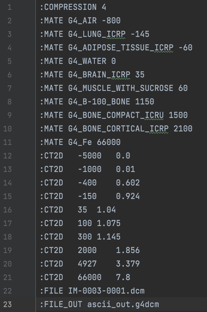
The first line gives the level of compression of the image. For example :COMPRESSION 4 means that only one slice
over four will be converted into the final voxelized geometry. The lines which start with :MATE give data
points for the HUs-to-materials curve, while the lines which start with :CT2D give data points for the
HUs-to-density curve. For each curve, a linear interpolation is done based on the data points to find the most
appropriate density and material for each voxel. The user must give the path to this file in the definition of the ct
element, as the parameter dicomDataFile. The user must also give the name of the dicom (.dcm) file to be converted.
This must be done with the flag :FILE, followed by the name of the file, which needs to be in the same folder
as the interpolation data file. The last flag :FILE_OUT is optional, and can be used to give a specific name to
the temporary output file which is generated during the conversion CT image.
An example of such a data file is provided in bdsim/examples/features/dicom/data.dat and can be used as a starting point.
Note
For a correct visualization of the DICOM image, a path to a colourMap.dat file must also be given,
as the parameter dicomDataPath. This file will allow the mapping of each material to a specific color in the
viewer. Its first line should bethe number of materials used in the simulation. Each material given in the
data.dat file should then have a colour scheme which the user defines via four numbers with the syntax
:1MAT X Y Z A where X, Y, Z and A are numbers between 0 and 1 respectively setting the amount of red, green,
blue and opacity of the colour defined for the material MAT. An example of such a colourMap.dat file is provided in
bdsim/examples/features/dicom/colourMap.dat.
Note
To be able to load CT images, BDSIM must be compiled with the USE_DICOM variable set to ON. Moreover, the conversion of the images requires the installation of the DCMTK package. This package is needed to easily extract the HUs data from the images. Information to download and install DCMTK can be found here: https://dicom.offis.de/dcmtk.php.en.
Examples:
DICOM: ct, l=1*m, dicomDataPath="./", dicomDataFile="data.dat";
Parameter |
Description |
l |
Length of the CT element along the beamline. |
dicomDataFile |
Name of the file which contains the conversion material-to-density and material-to-HU tables. |
dicomDataPath |
Path to the colourMap.dat file. During the conversion of the CT image, the temporary .g4dcm file will also be stored in this path. |
Offsets & Tilts - Component Misalignment
To simulate a real accelerator it may be necessary to introduce measured placement offsets or misalignments and rotations. Every component can be displaced transversely and rotated along the axis of the beam propagation.
Note
Components that have a finite angle (rbend and sbend) will only respond to tilt and not vertical or horizontal offsets. This is because these would change the length of the bend about its central axis. This is not currently handled but may be implemented in future releases.
Note
A tilt on a component with a finite angle causes the axis the angle is induced in (typically the y- axis) to be rotated without rotating the reference frame of the beam, i.e. a dipole with a \(\pi/2\) tilt will become a vertical bend without flipping x and y in the sampler or subsequent components. This matches the behaviour of MAD8 and MAD-X.
Note
A right-handed coordinate system is used and the beamline is built along the z direction.
Note
Tilts and offsets are independent of one another, that is to say, a tilt of \(\pi/2\) combined with a non-zero offsetX will not result in a vertical displacement.
The misalignments can be controlled through the following parameters.
Parameter |
Default value |
|---|---|
offsetX |
Horizontal displacement of the component [m] |
offsetY |
Vertical displacement of the component [m] |
tilt |
Clockwise rotation of the component, facing in the direction of the beamline z [rad]. In the case of an rbend or sbend, this rotates the axis about which the beam bends. |
Examples:
d1: drift, l=1*m, offsetX=1*cm;
d2: drift, l=0.5*m, offsetY = 0.3*cm, tilt=0.003;
Lattice Sequence
Once all the necessary components have been defined, they must be placed in a sequence to make a lattice. Elements can be repeated. A sequence of elements is defined by a line. Lines of lines can be made to describe the accelerator sequence programmatically, i.e.
d1: drift, l=3*m;
q1: quadrupole, l=0.1*m, k1=0.684;
q2: quadrupole, l=0.1*m, k1=-0.684;
fodo: line = (q1,d1,q2,d1);
transportline: line(fodo, fodo, fodo, fodo);
Line
line defines a sequence of elements.
name: line=(element1, element2, element3, ... );
Here, element can be any element or line. Lines can also be reversed using
line_name : line=-(line_2)
or within another line by:
line=(line_1,-line_2)
Reversing a line also reverses all nested lines within.
use - Defining which Line to Use
Once all elements and at least one line is defined, the main sequence of the beam line can be defined. This is defined using the following syntax:
use, period=<line_name>
Examples:
d1: drift, l=3.2*m;
q1: quadrupole, l=20*cm, k1=4.5;
q2: quadrupole, l=20*cm, k1=-4.5;
fodo: line=(d1,q1,d1,q2,d1);
use, period=fodo;
The beam line is placed in the world volume (the outermost coordinate system) starting at position (0,0,0) with direction (0,0,1) - i.e. pointing in positive z. The user may specify an initial offset and rotation for the beam line with respect to the world volume using the options described in Offset for Main Beam Line.
Warning
When the use command is called, the elements are copied internally,
so their definition is fixed. Any element parameter adjustments or redefinitions
after the use command will therefore not be observed.
Multiple beam lines may also be visualised - but only visualised (not suitable for simulations currently). Details are provided in Multiple Beam Lines.
Multiple Beam Lines
BDSIM has the ability to use multiple beam lines. This feature is still in development and is currently only for visualisation purposes. Secondary beam lines are placed either with respect to the world coordinate system or with respect to a particular element in the main beam line. A few caveats:
Only for visualisation purposes
Beam lines cannot be placed with respect to an element in another secondary beam line.
Secondary beam lines are not suitable for tracking.
Secondary beam lines are not sensitive to energy deposition, nor do they produce output.
The user is entirely responsible for overlapping geometry. The visualiser will render the geometry, but of course it will not be suitable for simulations, as overlaps lead to volume navigation problems and incorrect tracking.
The user may use any sequence defined in the parser before the use command. The secondary beam line is produced by declaring a placement. The placement definition (see Placements) is augmented with the following parameters:
Parameter |
Description |
|---|---|
sequence |
Name of the sequence (with line) to use for the secondary beam line |
referenceElement |
The element in the sequence with respect to which the beam line will be placed |
referenceElementNumber |
The i th instance of the element in the sequence (zero counting) ( i.e. 2 -> the 3rd instance of referenceElement in the sequence). |
Examples
This example is shown in bdsim/examples/features/geometry/10_multiple_beamlines. It defines a simple beam line and two other sequences that are placed alongside it. Further explanation is given below the example.
d1: drift, l=1*m;
d2: drift, l=3*m;
d3: drift, l=5*m;
sb1: sbend, l=1*m, angle=0.5;
sb2: sbend, l=1*m, angle=-0.5;
q1: quadrupole, l=0.2*m, k1=4.166666;
q2: quadrupole, l=0.2*m, k1=-4.166666;

fodo: line=(d1,q1,d1,q2);
mainLine: line=(d2,sb1,d2,sb2,d2,fodo,fodo);

auxLine1: line=(d3,sb1,d1,sb2,d1,fodo,d1);
auxLine2: line=(d1,sb1,d1,sb2,d1,fodo,d1);
auxLine3: line=(fodo);

use, mainLine;

beam, particle="e-",
      energy=3*GeV;

auxLine1Place: placement, sequence = "auxLine1",
                          referenceElement = "d2" ,
                          referenceElementNumber = 2,
                          x = -5*cm,
                          z = -1*m,
                          axisAngle = 1,
                          axisY = 1,
                          angle = -0.2;

auxLine2Place: placement, sequence = "auxLine2",
                          referenceElement = "d2",
                          referenceElementNumber = 2,
                          x = -10*cm,
                          z = -1*m,
                          axisAngle = 1,
                          axisY = 1,
                          angle = -0.5;

auxLine3Place: placement, sequence = "auxLine3",
                          x = 1*m,
                          axisAngle = 1,
                          axisY = 1,
                          angle = 0.2;
Firstly, a series of simple elements are defined (drifts, quadrupoles and bends). A simple sequence called fodo is defined and also the main beam line, called mainLine. After this, extra sequences are defined that we will use for secondary beam lines. The use command selects which beam line the simulation will be based on.
use, mainLine;
After this, the beam is defined (required for any simulation for rigidity calculations), then the placement of secondary beam lines.
The first placement auxLine1Place is a placement that will place the sequence named auxLine1 with respect to the third instance of the element d2 in the primary sequence (mainLine).
auxLine1Place: placement, sequence="auxLine1",
                          referenceElement="d2" ,
                          referenceElementNumber=2,
The placement is generally with respect to the centre of the element described in the primary beam line and along the direction it’s pointing. Without any displacement, the geometry would therefore overlap. Here, an offset and rotation are specified for this particular placement. An offset in x of -5 cm and -1 m in z is specified. The coordinate system is right-handed with positive-z pointing along the direction of travel in the beam line. A negative-x displacement is therefore to the right, looking along the direction of travel and 1 m in z is towards the beginning of the element from the centre. Rotations are described in Placements. Here, an axis angle rotation is used. The beam line is rotated about the unit Y-axis (local to that element) by -0.2 rad.
The second placement uses a different sequence, but in a similar fashion.
The third placement doesn’t specify a referenceElement, so the placement is with respect to the beginning of the beam line.
The model is shown below.
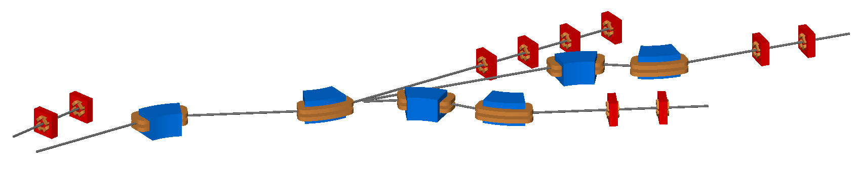
The drift segments do not of course connect but are merely placed close to each other. In future, continuous vacuum points will be provided.
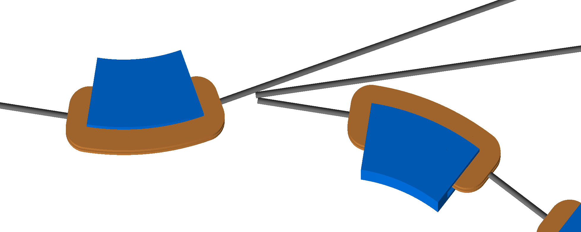
Detectors
BDSIM allows the definition of detectors in the simulation. These are objects to represent real detectors or measure a quantity at some place in the model including the effect of the mass of (and therefore interaction with) the detector. Currently, there is one type of detector that is a beam loss monitor.
Beam Loss Monitors
Beam loss monitors (BLMs) are simple detectors that give one integrated value per event. The quantity to be generated can be chosen and the shape and location of the BLM can also be chosen. Below are the available parameters. A BLM is created using the blm command.:
detectorname, blm, parameter=value...
Either a simple geometric shape can be used, which is a single volume of one material, or a user supplied geometry file can be used.
The quantity produced by the BLM per event is defined using a scorer (see Scorer) and attached to the BLM with the scoreQuantity parameter. If this is not defined, it is simply passive material.
The BLM signals are put in a 1D histogram for each scorer used with any BLM where each bin is a BLM in order it appears in construction. If a certain scorer isn’t attached to a BLM, the corresponding bin in that scorer histogram will always be 0. The best way to view the BLM signals from a run is to use rebdsimHistoMerge as described in Quick Recipes. See also BLM Output.
The placement parameters are the same as the general placements (see Placements). So the BLM can be placed with respect to a beam line element or generally in curvilinear coordinates, or in global Cartesian coordinates.
Bias objects may be attached to a BLM via the bias attribute. This names a defined
bias object (see Cross-Section Biasing). This is applied to all logical
volumes in the BLM.
Note
If multiple BLMs use the same external geometry file, the biasing will be applied to all of them as there is only one copy of the geometry in memory.
Parameter |
Description |
geometryType |
Name of simple geometry to use (“cylinder”, “cube”, “sphere”) |
blmMaterial |
Name of material to use for simple geometry |
blm1 |
BLM shape parameter 1 - different depending on the shape used |
blm2 |
BLM shape parameter 2 |
blm3 |
BLM shape parameter 2 |
blm4 |
BLM shape parameter 2 |
scoreQuantity |
Name of a scorer object that should be used for record a quantity in the BLM. See Scorer. |
x |
Offset in global x |
y |
Offset in global y |
z |
Offset in global z |
s |
Curvilinear s coordinate (global | local depending on parameters) |
phi |
Euler angle phi for rotation |
theta |
Euler angle theta for rotation |
psi |
Euler angle psi for rotation |
axisX |
Axis angle rotation x-component of unit vector |
axisY |
Axis angle rotation y-component of unit vector |
axisZ |
Axis angle rotation z-component of unit vector |
angle |
Axis angle, angle to rotate about unit vector |
axisAngle |
Boolean whether to use axis angle rotation scheme (default false) |
referenceElement |
Name of element to place geometry with respect to (string) |
referenceElementNumber |
Occurrence of referenceElement to place with respect to if it is used more than once in the sequence. Zero counting. |
geometryFile |
Optional file to use for geometry of BLM including format |
side |
Optional which side of referenceElement the BLM is placed with
respect to. One of |
sideOffset |
Distance from the (square) extent of an object the BLM is placed. |
bias |
Name of bias object to apply to all volumes in the BLM. |
BLM Shapes
For each shape, the shape parameters (“blm1”, “blm2”, “blm3”, “blm4”) have different meanings. These are described below. NA means non-applicable to this shape.
Shape |
blm1 |
blm2 |
blm3 |
blm4 |
|---|---|---|---|---|
cylinder |
half length along axis |
radius |
NA |
NA |
cube |
half length in x |
half length in y |
half length in z |
NA |
sphere |
radius |
NA |
NA |
NA |
BLM Output
BLM signals (integrals / scores per event per BLM) are stored in 1D histograms alongside other 1D
histograms such as the usual energy deposition histogram. There is 1 histogram per scorer used in any
BLM. All BLM histograms have the same number of bins which is the total number of BLMs in the model and
they are in the order they are constructed in the input. Here is an example that will clarify. This
example can be found in bdsim/examples/features/detectors/blms/blm-output-example.gmad.
r1: rcol, l=10*m, horizontalWidth=1*cm, material="Al";
l1: line=(r1);
use, l1;

beam, particle="e-",
      energy=10*GeV;

option, physicsList="em";

chrg: scorer, type="cellcharge";
dose: scorer, type="depositeddose";
eDep: scorer, type="depositedenergy";

BLM_t1: blm, s=10*cm,
             side="top",
             geometryType="cylinder",
             blmMaterial="Al",
             blm1=2*cm,
             blm2=1*cm,
             scoreQuantity="eDep dose chrg";

BLM_t2: blm, s=5*cm,
             side="left",
             geometryType="cylinder",
             blmMaterial="Al",
             blm1=2*cm,
             blm2=1*cm,
             scoreQuantity="dose eDep";

BLM_t3: blm, s=30*cm,
             side="top",
             geometryType="cylinder",
             blmMaterial="Al",
             blm1=2*cm,
             blm2=1*cm,
             scoreQuantity="chrg dose";
This model creates a scene with 1x 10m long block of aluminium (a closed rcol) and a beam of 10 GeV electrons fired into it. 3 different scorers are used (“chrg”, “dose” and “eDep”). However, only 1 BLM (“BLM_t1”) uses all 3.
The output will contain 3 histograms (1 for each scorer used with a BLM) containing 3 bins (1 for each BLM). The histograms will be called “BLM_chrg”, “BLM_dose” and “BLM_eDep”. The second bin of the BLM_chrg histogram (bin index #1) will always be 0 as the 2nd BLM (in order of construction) “BLM_t2” does not use the “chrg” scorer. This is done so that a given BLM is always in the same bin in all BLM histograms.
Note
The 2nd bin in each output histogram (bin index #1) will be for “BLM_t2” as it is the second to be constructed, even though it is placed geometrically before “BLM_t1” with respect to the beam line (s = 5cm vs s = 10cm).
The model was run with 10 events and the output summarised using rebdsimHistoMerge.
bdsim --file=blm-output-example.gmad --outfile=t1 --batch --ngenerate=10
rebdsimHistoMerge t1.root t1-histos.root
root -l t1-histos.root
> TBrowser tb;
Preview of “eDep” scorer histogram for all BLMs from above example. 3rd bin is empty as the 3rd BLM doesn’t use this scorer.
Preview of “dose” scorer histogram for all BLMs from above example. All bins are filled as all BLMs use this scorer.
Examples
A simple sphere made of nitrogen. It’s placed at 2.3 metres along the beam line with a transverse offset (in curvilinear coordinates) of 40 cm horizontally and 25 cm vertically. The sphere radius is 20 cm.
minidetector: blm, s=2.3*m, x=0.4*m, y=0.25*m,
              geometryType="sphere",
              blmMaterial="N",
              blm1=20*cm;
A simple cylinder made of silicon. It’s placed globally with an offset in x of 3.2 m and y of 25 cm.
minidetector: blm, x=3.2*m, y=0.25*m,
              geometryType="cylinder",
              blmMaterial="Si",
              blm1=20*cm,
              blm2=5*cm;
User defined geometry in a GDML file.
blmdose: scorer, type="depositedenery";
minidetector: blm, x=0.4*m, y=0.25*m,
              geometryFile="gdml:simpleshape.gdml",
              blmMaterial="N",
              blm1=20*cm,
              blm2=5*cm,
              scorerQuantity="blmdose";